You are viewing a plain text version of this content. The canonical link for it is here.
Posted to commits@mxnet.apache.org by in...@apache.org on 2018/06/26 16:54:22 UTC
[incubator-mxnet] branch master updated: [MXNET-593] Adding 2
tutorials on Learning Rate Schedules (#11296)
This is an automated email from the ASF dual-hosted git repository.
indhub pushed a commit to branch master
in repository https://gitbox.apache.org/repos/asf/incubator-mxnet.git
The following commit(s) were added to refs/heads/master by this push:
new e494cee [MXNET-593] Adding 2 tutorials on Learning Rate Schedules (#11296)
e494cee is described below
commit e494cee9b540eb19cc0220cc3b3dbfde074b55c9
Author: Thom Lane <th...@gmail.com>
AuthorDate: Tue Jun 26 09:54:06 2018 -0700
[MXNET-593] Adding 2 tutorials on Learning Rate Schedules (#11296)
* Added two tutorials on learning rate schedules; basic and advanced.
* Correcting notebook skip line.
* Corrected cosine graph
* Changes based on @KellenSunderland feedback.
---
docs/tutorials/gluon/learning_rate_schedules.md | 328 +++++++++++++++++++++
.../gluon/learning_rate_schedules_advanced.md | 308 +++++++++++++++++++
docs/tutorials/index.md | 2 +
tests/tutorials/test_tutorials.py | 14 +-
4 files changed, 648 insertions(+), 4 deletions(-)
diff --git a/docs/tutorials/gluon/learning_rate_schedules.md b/docs/tutorials/gluon/learning_rate_schedules.md
new file mode 100644
index 0000000..dc340b7
--- /dev/null
+++ b/docs/tutorials/gluon/learning_rate_schedules.md
@@ -0,0 +1,328 @@
+
+# Learning Rate Schedules
+
+Setting the learning rate for stochastic gradient descent (SGD) is crucially important when training neural networks because it controls both the speed of convergence and the ultimate performance of the network. One of the simplest learning rate strategies is to have a fixed learning rate throughout the training process. Choosing a small learning rate allows the optimizer find good solutions, but this comes at the expense of limiting the initial speed of convergence. Changing the learnin [...]
+
+Schedules define how the learning rate changes over time and are typically specified for each epoch or iteration (i.e. batch) of training. Schedules differ from adaptive methods (such as AdaDelta and Adam) because they:
+
+* change the global learning rate for the optimizer, rather than parameter-wise learning rates
+* don't take feedback from the training process and are specified beforehand
+
+In this tutorial, we visualize the schedules defined in `mx.lr_scheduler`, show how to implement custom schedules and see an example of using a schedule while training models. Since schedules are passed to `mx.optimizer.Optimizer` classes, these methods work with both Module and Gluon APIs.
+
+
+```python
+%matplotlib inline
+from __future__ import print_function
+import math
+import matplotlib.pyplot as plt
+import mxnet as mx
+from mxnet.gluon import nn
+from mxnet.gluon.data.vision import transforms
+import numpy as np
+```
+
+```python
+def plot_schedule(schedule_fn, iterations=1500):
+ # Iteration count starting at 1
+ iterations = [i+1 for i in range(iterations)]
+ lrs = [schedule_fn(i) for i in iterations]
+ plt.scatter(iterations, lrs)
+ plt.xlabel("Iteration")
+ plt.ylabel("Learning Rate")
+ plt.show()
+```
+
+## Schedules
+
+In this section, we take a look at the schedules in `mx.lr_scheduler`. All of these schedules define the learning rate for a given iteration, and it is expected that iterations start at 1 rather than 0. So to find the learning rate for the 100th iteration, you can call `schedule(100)`.
+
+### Stepwise Decay Schedule
+
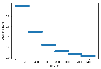
+One of the most commonly used learning rate schedules is called stepwise decay, where the learning rate is reduced by a factor at certain intervals. MXNet implements a `FactorScheduler` for equally spaced intervals, and `MultiFactorScheduler` for greater control. We start with an example of halving the learning rate every 250 iterations. More precisely, the learning rate will be multiplied by `factor` _after_ the `step` index and multiples thereafter. So in the example below the learning [...]
+
+
+```python
+schedule = mx.lr_scheduler.FactorScheduler(step=250, factor=0.5)
+schedule.base_lr = 1
+plot_schedule(schedule)
+```
+
+
+ <!--notebook-skip-line-->
+
+
+Note: the `base_lr` is used to determine the initial learning rate. It takes a default value of 0.01 since we inherit from `mx.lr_scheduler.LRScheduler`, but it can be set as a property of the schedule. We will see later in this tutorial that `base_lr` is set automatically when providing the `lr_schedule` to `Optimizer`. Also be aware that the schedules in `mx.lr_scheduler` have state (i.e. counters, etc) so calling the schedule out of order may give unexpected results.
+
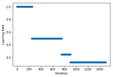
+We can define non-uniform intervals with `MultiFactorScheduler` and in the example below we halve the learning rate _after_ the 250th, 750th (i.e. a step length of 500 iterations) and 900th (a step length of 150 iterations). As before, the learning rate of the 250th iteration will be 1 and the 251th iteration will be 0.5.
+
+
+```python
+schedule = mx.lr_scheduler.MultiFactorScheduler(step=[250, 750, 900], factor=0.5)
+schedule.base_lr = 1
+plot_schedule(schedule)
+```
+
+
+ <!--notebook-skip-line-->
+
+
+### Polynomial Schedule
+
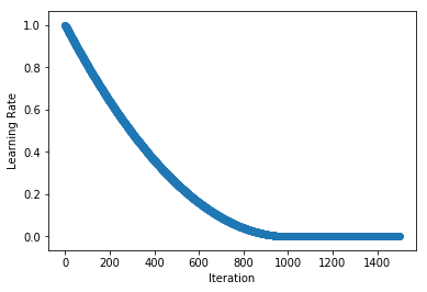
+Stepwise schedules and the discontinuities they introduce may sometimes lead to instability in the optimization, so in some cases smoother schedules are preferred. `PolyScheduler` gives a smooth decay using a polynomial function and reaches a learning rate of 0 after `max_update` iterations. In the example below, we have a quadratic function (`pwr=2`) that falls from 0.998 at iteration 1 to 0 at iteration 1000. After this the learning rate stays at 0, so nothing will be learnt from `max_ [...]
+
+
+```python
+schedule = mx.lr_scheduler.PolyScheduler(max_update=1000, base_lr=1, pwr=2)
+plot_schedule(schedule)
+```
+
+
+ <!--notebook-skip-line-->
+
+
+Note: unlike `FactorScheduler`, the `base_lr` is set as an argument when instantiating the schedule.
+
+And we don't evaluate at `iteration=0` (to get `base_lr`) since we are working with schedules starting at `iteration=1`.
+
+### Custom Schedules
+
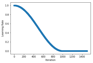
+You can implement your own custom schedule with a function or callable class, that takes an integer denoting the iteration index (starting at 1) and returns a float representing the learning rate to be used for that iteration. We implement the Cosine Annealing Schedule in the example below as a callable class (see `__call__` method).
+
+
+```python
+class CosineAnnealingSchedule():
+ def __init__(self, min_lr, max_lr, cycle_length):
+ self.min_lr = min_lr
+ self.max_lr = max_lr
+ self.cycle_length = cycle_length
+
+ def __call__(self, iteration):
+ if iteration <= self.cycle_length:
+ unit_cycle = (1 + math.cos(iteration * math.pi / self.cycle_length)) / 2
+ adjusted_cycle = (unit_cycle * (self.max_lr - self.min_lr)) + self.min_lr
+ return adjusted_cycle
+ else:
+ return self.min_lr
+
+
+schedule = CosineAnnealingSchedule(min_lr=0, max_lr=1, cycle_length=1000)
+plot_schedule(schedule)
+```
+
+
+ <!--notebook-skip-line-->
+
+
+## Using Schedules
+
+While training a simple handwritten digit classifier on the MNIST dataset, we take a look at how to use a learning rate schedule during training. Our demonstration model is a basic convolutional neural network. We start by preparing our `DataLoader` and defining the network.
+
+As discussed above, the schedule should return a learning rate given an (1-based) iteration index.
+
+
+```python
+# Use GPU if one exists, else use CPU
+ctx = mx.gpu() if mx.test_utils.list_gpus() else mx.cpu()
+
+# MNIST images are 28x28. Total pixels in input layer is 28x28 = 784
+num_inputs = 784
+# Clasify the images into one of the 10 digits
+num_outputs = 10
+# 64 images in a batch
+batch_size = 64
+
+# Load the training data
+train_dataset = mx.gluon.data.vision.MNIST(train=True).transform_first(transforms.ToTensor())
+train_dataloader = mx.gluon.data.DataLoader(train_dataset, batch_size, shuffle=True)
+
+# Build a simple convolutional network
+def build_cnn():
+ net = nn.HybridSequential()
+ with net.name_scope():
+ # First convolution
+ net.add(nn.Conv2D(channels=10, kernel_size=5, activation='relu'))
+ net.add(nn.MaxPool2D(pool_size=2, strides=2))
+ # Second convolution
+ net.add(nn.Conv2D(channels=20, kernel_size=5, activation='relu'))
+ net.add(nn.MaxPool2D(pool_size=2, strides=2))
+ # Flatten the output before the fully connected layers
+ net.add(nn.Flatten())
+ # First fully connected layers with 512 neurons
+ net.add(nn.Dense(512, activation="relu"))
+ # Second fully connected layer with as many neurons as the number of classes
+ net.add(nn.Dense(num_outputs))
+ return net
+
+net = build_cnn()
+```
+
+We then initialize our network (technically deferred until we pass the first batch) and define the loss.
+
+
+```python
+# Initialize the parameters with Xavier initializer
+net.collect_params().initialize(mx.init.Xavier(), ctx=ctx)
+# Use cross entropy loss
+softmax_cross_entropy = mx.gluon.loss.SoftmaxCrossEntropyLoss()
+```
+
+We're now ready to create our schedule, and in this example we opt for a stepwise decay schedule using `MultiFactorScheduler`. Since we're only training a demonstration model for a limited number of epochs (10 in total) we will exaggerate the schedule and drop the learning rate by 90% after the 4th, 7th and 9th epochs. We call these steps, and the drop occurs _after_ the step index. Schedules are defined for iterations (i.e. training batches), so we must represent our steps in iterations too.
+
+
+```python
+steps_epochs = [4, 7, 9]
+# assuming we keep partial batches, see `last_batch` parameter of DataLoader
+iterations_per_epoch = math.ceil(len(train_dataset) / batch_size)
+# iterations just before starts of epochs (iterations are 1-indexed)
+steps_iterations = [s*iterations_per_epoch for s in steps_epochs]
+print("Learning rate drops after iterations: {}".format(steps_iterations))
+```
+
+ Learning rate drops after iterations: [3752, 6566, 8442]
+
+
+
+```python
+schedule = mx.lr_scheduler.MultiFactorScheduler(step=steps_iterations, factor=0.1)
+```
+
+**We create our `Optimizer` and pass the schedule via the `lr_scheduler` parameter.** In this example we're using Stochastic Gradient Descent.
+
+
+```python
+sgd_optimizer = mx.optimizer.SGD(learning_rate=0.03, lr_scheduler=schedule)
+```
+
+And we use this optimizer (with schedule) in our `Trainer` and train for 10 epochs. Alternatively, we could have set the `optimizer` to the string `sgd`, and pass a dictionary of the optimizer parameters directly to the trainer using `optimizer_params`.
+
+
+```python
+trainer = mx.gluon.Trainer(params=net.collect_params(), optimizer=sgd_optimizer)
+```
+
+
+```python
+num_epochs = 10
+# epoch and batch counts starting at 1
+for epoch in range(1, num_epochs+1):
+ # Iterate through the images and labels in the training data
+ for batch_num, (data, label) in enumerate(train_dataloader, start=1):
+ # get the images and labels
+ data = data.as_in_context(ctx)
+ label = label.as_in_context(ctx)
+ # Ask autograd to record the forward pass
+ with mx.autograd.record():
+ # Run the forward pass
+ output = net(data)
+ # Compute the loss
+ loss = softmax_cross_entropy(output, label)
+ # Compute gradients
+ loss.backward()
+ # Update parameters
+ trainer.step(data.shape[0])
+
+ # Show loss and learning rate after first iteration of epoch
+ if batch_num == 1:
+ curr_loss = mx.nd.mean(loss).asscalar()
+ curr_lr = trainer.learning_rate
+ print("Epoch: %d; Batch %d; Loss %f; LR %f" % (epoch, batch_num, curr_loss, curr_lr))
+```
+
+Epoch: 1; Batch 1; Loss 2.304071; LR 0.030000 <!--notebook-skip-line-->
+
+Epoch: 2; Batch 1; Loss 0.059640; LR 0.030000 <!--notebook-skip-line-->
+
+Epoch: 3; Batch 1; Loss 0.072601; LR 0.030000 <!--notebook-skip-line-->
+
+Epoch: 4; Batch 1; Loss 0.042228; LR 0.030000 <!--notebook-skip-line-->
+
+Epoch: 5; Batch 1; Loss 0.025745; LR 0.003000 <!--notebook-skip-line-->
+
+Epoch: 6; Batch 1; Loss 0.027391; LR 0.003000 <!--notebook-skip-line-->
+
+Epoch: 7; Batch 1; Loss 0.048237; LR 0.003000 <!--notebook-skip-line-->
+
+Epoch: 8; Batch 1; Loss 0.024213; LR 0.000300 <!--notebook-skip-line-->
+
+Epoch: 9; Batch 1; Loss 0.008892; LR 0.000300 <!--notebook-skip-line-->
+
+Epoch: 10; Batch 1; Loss 0.006875; LR 0.000030 <!--notebook-skip-line-->
+
+
+We see that the learning rate starts at 0.03, and falls to 0.00003 by the end of training as per the schedule we defined.
+
+### Manually setting the learning rate: Gluon API only
+
+When using the method above you don't need to manually keep track of iteration count and set the learning rate, so this is the recommended approach for most cases. Sometimes you might want more fine-grained control over setting the learning rate though, so Gluon's `Trainer` provides the `set_learning_rate` method for this.
+
+We replicate the example above, but now keep track of the `iteration_idx`, call the schedule and set the learning rate appropriately using `set_learning_rate`. We also use `schedule.base_lr` to set the initial learning rate for the schedule since we are calling the schedule directly and not using it as part of the `Optimizer`.
+
+
+```python
+net = build_cnn()
+net.collect_params().initialize(mx.init.Xavier(), ctx=ctx)
+
+schedule = mx.lr_scheduler.MultiFactorScheduler(step=steps_iterations, factor=0.1)
+schedule.base_lr = 0.03
+sgd_optimizer = mx.optimizer.SGD()
+trainer = mx.gluon.Trainer(params=net.collect_params(), optimizer=sgd_optimizer)
+
+iteration_idx = 1
+num_epochs = 10
+# epoch and batch counts starting at 1
+for epoch in range(1, num_epochs + 1):
+ # Iterate through the images and labels in the training data
+ for batch_num, (data, label) in enumerate(train_dataloader, start=1):
+ # get the images and labels
+ data = data.as_in_context(ctx)
+ label = label.as_in_context(ctx)
+ # Ask autograd to record the forward pass
+ with mx.autograd.record():
+ # Run the forward pass
+ output = net(data)
+ # Compute the loss
+ loss = softmax_cross_entropy(output, label)
+ # Compute gradients
+ loss.backward()
+ # Update the learning rate
+ lr = schedule(iteration_idx)
+ trainer.set_learning_rate(lr)
+ # Update parameters
+ trainer.step(data.shape[0])
+ # Show loss and learning rate after first iteration of epoch
+ if batch_num == 1:
+ curr_loss = mx.nd.mean(loss).asscalar()
+ curr_lr = trainer.learning_rate
+ print("Epoch: %d; Batch %d; Loss %f; LR %f" % (epoch, batch_num, curr_loss, curr_lr))
+ iteration_idx += 1
+```
+
+Epoch: 1; Batch 1; Loss 2.334119; LR 0.030000 <!--notebook-skip-line-->
+
+Epoch: 2; Batch 1; Loss 0.178930; LR 0.030000 <!--notebook-skip-line-->
+
+Epoch: 3; Batch 1; Loss 0.142640; LR 0.030000 <!--notebook-skip-line-->
+
+Epoch: 4; Batch 1; Loss 0.041116; LR 0.030000 <!--notebook-skip-line-->
+
+Epoch: 5; Batch 1; Loss 0.051049; LR 0.003000 <!--notebook-skip-line-->
+
+Epoch: 6; Batch 1; Loss 0.027170; LR 0.003000 <!--notebook-skip-line-->
+
+Epoch: 7; Batch 1; Loss 0.083776; LR 0.003000 <!--notebook-skip-line-->
+
+Epoch: 8; Batch 1; Loss 0.082553; LR 0.000300 <!--notebook-skip-line-->
+
+Epoch: 9; Batch 1; Loss 0.027984; LR 0.000300 <!--notebook-skip-line-->
+
+Epoch: 10; Batch 1; Loss 0.030896; LR 0.000030 <!--notebook-skip-line-->
+
+
+Once again, we see the learning rate start at 0.03, and fall to 0.00003 by the end of training as per the schedule we defined.
+
+## Advanced Schedules
+
+We have a related tutorial on Advanced Learning Rate Schedules that shows reference implementations of schedules that give state-of-the-art results. We look at cyclical schedules applied to a variety of cycle shapes, and many other techniques such as warm-up and cool-down.
+
+<!-- INSERT SOURCE DOWNLOAD BUTTONS -->
\ No newline at end of file
diff --git a/docs/tutorials/gluon/learning_rate_schedules_advanced.md b/docs/tutorials/gluon/learning_rate_schedules_advanced.md
new file mode 100644
index 0000000..bdaf0a9
--- /dev/null
+++ b/docs/tutorials/gluon/learning_rate_schedules_advanced.md
@@ -0,0 +1,308 @@
+
+ # Advanced Learning Rate Schedules
+
+Given the importance of learning rate and the learning rate schedule for training neural networks, there have been a number of research papers published recently on the subject. Although many practitioners are using simple learning rate schedules such as stepwise decay, research has shown that there are other strategies that work better in most situations. We implement a number of different schedule shapes in this tutorial and introduce cyclical schedules.
+
+See the "Learning Rate Schedules" tutorial for a more basic overview of learning rates, and an example of how to use them while training your own models.
+
+
+```python
+%matplotlib inline
+import copy
+import math
+import mxnet as mx
+import numpy as np
+import matplotlib.pyplot as plt
+```
+
+```python
+def plot_schedule(schedule_fn, iterations=1500):
+ # Iteration count starting at 1
+ iterations = [i+1 for i in range(iterations)]
+ lrs = [schedule_fn(i) for i in iterations]
+ plt.scatter(iterations, lrs)
+ plt.xlabel("Iteration")
+ plt.ylabel("Learning Rate")
+ plt.show()
+```
+
+## Custom Schedule Shapes
+
+### (Slanted) Triangular
+
+While trying to push the boundaries of batch size for faster training, [Priya Goyal et al. (2017)](https://arxiv.org/abs/1706.02677) found that having a smooth linear warm up in the learning rate at the start of training improved the stability of the optimizer and lead to better solutions. It was found that a smooth increases gave improved performance over stepwise increases.
+
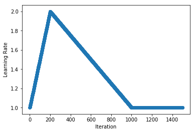
+We look at "warm-up" in more detail later in the tutorial, but this could be viewed as a specific case of the **"triangular"** schedule that was proposed by [Leslie N. Smith (2015)](https://arxiv.org/abs/1506.01186). Quite simply, the schedule linearly increases then decreases between a lower and upper bound. Originally it was suggested this schedule be used as part of a cyclical schedule but more recently researchers have been using a single cycle.
+
+One adjustment proposed by [Jeremy Howard, Sebastian Ruder (2018)](https://arxiv.org/abs/1801.06146) was to change the ratio between the increasing and decreasing stages, instead of the 50:50 split. Changing the increasing fraction (`inc_fraction!=0.5`) leads to a **"slanted triangular"** schedule. Using `inc_fraction<0.5` tends to give better results.
+
+
+```python
+class TriangularSchedule():
+ def __init__(self, min_lr, max_lr, cycle_length, inc_fraction=0.5):
+ """
+ min_lr: lower bound for learning rate (float)
+ max_lr: upper bound for learning rate (float)
+ cycle_length: iterations between start and finish (int)
+ inc_fraction: fraction of iterations spent in increasing stage (float)
+ """
+ self.min_lr = min_lr
+ self.max_lr = max_lr
+ self.cycle_length = cycle_length
+ self.inc_fraction = inc_fraction
+
+ def __call__(self, iteration):
+ if iteration <= self.cycle_length*self.inc_fraction:
+ unit_cycle = iteration * 1 / (self.cycle_length * self.inc_fraction)
+ elif iteration <= self.cycle_length:
+ unit_cycle = (self.cycle_length - iteration) * 1 / (self.cycle_length * (1 - self.inc_fraction))
+ else:
+ unit_cycle = 0
+ adjusted_cycle = (unit_cycle * (self.max_lr - self.min_lr)) + self.min_lr
+ return adjusted_cycle
+```
+
+We look an example of a slanted triangular schedule that increases from a learning rate of 1 to 2, and back to 1 over 1000 iterations. Since we set `inc_fraction=0.2`, 200 iterations are used for the increasing stage, and 800 for the decreasing stage. After this, the schedule stays at the lower bound indefinitely.
+
+
+```python
+schedule = TriangularSchedule(min_lr=1, max_lr=2, cycle_length=1000, inc_fraction=0.2)
+plot_schedule(schedule)
+```
+
+
+ <!--notebook-skip-line-->
+
+
+### Cosine
+
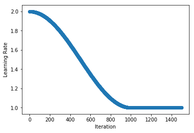
+Continuing with the idea that smooth decay profiles give improved performance over stepwise decay, [Ilya Loshchilov, Frank Hutter (2016)](https://arxiv.org/abs/1608.03983) used **"cosine annealing"** schedules to good effect. As with triangular schedules, the original idea was that this should be used as part of a cyclical schedule, but we begin by implementing the cosine annealing component before the full Stochastic Gradient Descent with Warm Restarts (SGDR) method later in the tutorial.
+
+
+```python
+class CosineAnnealingSchedule():
+ def __init__(self, min_lr, max_lr, cycle_length):
+ """
+ min_lr: lower bound for learning rate (float)
+ max_lr: upper bound for learning rate (float)
+ cycle_length: iterations between start and finish (int)
+ """
+ self.min_lr = min_lr
+ self.max_lr = max_lr
+ self.cycle_length = cycle_length
+
+ def __call__(self, iteration):
+ if iteration <= self.cycle_length:
+ unit_cycle = (1 + math.cos(iteration * math.pi / self.cycle_length)) / 2
+ adjusted_cycle = (unit_cycle * (self.max_lr - self.min_lr)) + self.min_lr
+ return adjusted_cycle
+ else:
+ return self.min_lr
+```
+
+We look at an example of a cosine annealing schedule that smoothing decreases from a learning rate of 2 to 1 across 1000 iterations. After this, the schedule stays at the lower bound indefinietly.
+
+
+```python
+schedule = CosineAnnealingSchedule(min_lr=1, max_lr=2, cycle_length=1000)
+plot_schedule(schedule)
+```
+
+
+ <!--notebook-skip-line-->
+
+
+## Custom Schedule Modifiers
+
+We now take a look some adjustments that can be made to existing schedules. We see how to add linear warm-up and its compliment linear cool-down, before using this to implement the "1-Cycle" schedule used by [Leslie N. Smith, Nicholay Topin (2017)](https://arxiv.org/abs/1708.07120) for "super-convergence". We then look at cyclical schedules and implement the original cyclical schedule from [Leslie N. Smith (2015)](https://arxiv.org/abs/1506.01186) before finishing with a look at ["SGDR: [...]
+
+Unlike the schedules above and those implemented in `mx.lr_scheduler`, these classes are designed to modify existing schedules so they take the argument `schedule` (for initialized schedules) or `schedule_class` when being initialized.
+
+### Warm-Up
+
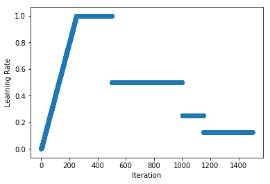
+Using the idea of linear warm-up of the learning rate proposed in ["Accurate, Large Minibatch SGD: Training ImageNet in 1 Hour" by Priya Goyal et al. (2017)](https://arxiv.org/abs/1706.02677), we implement a wrapper class that adds warm-up to an existing schedule. Going from `start_lr` to the initial learning rate of the `schedule` over `length` iterations, this adjustment is useful when training with large batch sizes.
+
+
+```python
+class LinearWarmUp():
+ def __init__(self, schedule, start_lr, length):
+ """
+ schedule: a pre-initialized schedule (e.g. TriangularSchedule(min_lr=0.5, max_lr=2, cycle_length=500))
+ start_lr: learning rate used at start of the warm-up (float)
+ length: number of iterations used for the warm-up (int)
+ """
+ self.schedule = schedule
+ self.start_lr = start_lr
+ # calling mx.lr_scheduler.LRScheduler effects state, so calling a copy
+ self.finish_lr = copy.copy(schedule)(0)
+ self.length = length
+
+ def __call__(self, iteration):
+ if iteration <= self.length:
+ return iteration * (self.finish_lr - self.start_lr)/(self.length) + self.start_lr
+ else:
+ return self.schedule(iteration - self.length)
+```
+
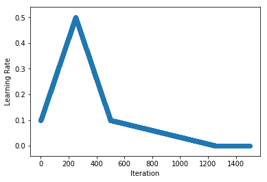
+As an example, we add a linear warm-up of the learning rate (from 0 to 1 over 250 iterations) to a stepwise decay schedule. We first create the `MultiFactorScheduler` (and set the `base_lr`) and then pass it to `LinearWarmUp` to add the warm-up at the start. We can use `LinearWarmUp` with any other schedule including `CosineAnnealingSchedule`.
+
+
+```python
+schedule = mx.lr_scheduler.MultiFactorScheduler(step=[250, 750, 900], factor=0.5)
+schedule.base_lr = 1
+schedule = LinearWarmUp(schedule, start_lr=0, length=250)
+plot_schedule(schedule)
+```
+
+
+ <!--notebook-skip-line-->
+
+
+### Cool-Down
+
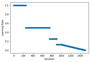
+Similarly, we could add a linear cool-down period to our schedule and this is used in the "1-Cycle" schedule proposed by [Leslie N. Smith, Nicholay Topin (2017)](https://arxiv.org/abs/1708.07120) to train neural networks very quickly in certain circumstances (coined "super-convergence"). We reduce the learning rate from its value at `start_idx` of `schedule` to `finish_lr` over a period of `length`, and then maintain `finish_lr` thereafter.
+
+
+```python
+class LinearCoolDown():
+ def __init__(self, schedule, finish_lr, start_idx, length):
+ """
+ schedule: a pre-initialized schedule (e.g. TriangularSchedule(min_lr=0.5, max_lr=2, cycle_length=500))
+ finish_lr: learning rate used at end of the cool-down (float)
+ start_idx: iteration to start the cool-down (int)
+ length: number of iterations used for the cool-down (int)
+ """
+ self.schedule = schedule
+ # calling mx.lr_scheduler.LRScheduler effects state, so calling a copy
+ self.start_lr = copy.copy(self.schedule)(start_idx)
+ self.finish_lr = finish_lr
+ self.start_idx = start_idx
+ self.finish_idx = start_idx + length
+ self.length = length
+
+ def __call__(self, iteration):
+ if iteration <= self.start_idx:
+ return self.schedule(iteration)
+ elif iteration <= self.finish_idx:
+ return (iteration - self.start_idx) * (self.finish_lr - self.start_lr) / (self.length) + self.start_lr
+ else:
+ return self.finish_lr
+```
+
+As an example, we apply learning rate cool-down to a `MultiFactorScheduler`. Starting the cool-down at iteration 1000, we reduce the learning rate linearly from 0.125 to 0.001 over 500 iterations, and hold the learning rate at 0.001 after this.
+
+
+```python
+schedule = mx.lr_scheduler.MultiFactorScheduler(step=[250, 750, 900], factor=0.5)
+schedule.base_lr = 1
+schedule = LinearCoolDown(schedule, finish_lr=0.001, start_idx=1000, length=500)
+plot_schedule(schedule)
+```
+
+
+ <!--notebook-skip-line-->
+
+
+#### 1-Cycle: for "Super-Convergence"
+
+So we can implement the "1-Cycle" schedule proposed by [Leslie N. Smith, Nicholay Topin (2017)](https://arxiv.org/abs/1708.07120) we use a single and symmetric cycle of the triangular schedule above (i.e. `inc_fraction=0.5`), followed by a cool-down period of `cooldown_length` iterations.
+
+
+```python
+class OneCycleSchedule():
+ def __init__(self, start_lr, max_lr, cycle_length, cooldown_length=0, finish_lr=None):
+ """
+ start_lr: lower bound for learning rate in triangular cycle (float)
+ max_lr: upper bound for learning rate in triangular cycle (float)
+ cycle_length: iterations between start and finish of triangular cycle: 2x 'stepsize' (int)
+ cooldown_length: number of iterations used for the cool-down (int)
+ finish_lr: learning rate used at end of the cool-down (float)
+ """
+ if (cooldown_length > 0) and (finish_lr is None):
+ raise ValueError("Must specify finish_lr when using cooldown_length > 0.")
+ if (cooldown_length == 0) and (finish_lr is not None):
+ raise ValueError("Must specify cooldown_length > 0 when using finish_lr.")
+
+ finish_lr = finish_lr if (cooldown_length > 0) else start_lr
+ schedule = TriangularSchedule(min_lr=start_lr, max_lr=max_lr, cycle_length=cycle_length)
+ self.schedule = LinearCoolDown(schedule, finish_lr=finish_lr, start_idx=cycle_length, length=cooldown_length)
+
+ def __call__(self, iteration):
+ return self.schedule(iteration)
+```
+
+As an example, we linearly increase and then decrease the learning rate from 0.1 to 0.5 and back over 500 iterations (i.e. single triangular cycle), before reducing the learning rate further to 0.001 over the next 750 iterations (i.e. cool-down).
+
+
+```python
+schedule = OneCycleSchedule(start_lr=0.1, max_lr=0.5, cycle_length=500, cooldown_length=750, finish_lr=0.001)
+plot_schedule(schedule)
+```
+
+
+ <!--notebook-skip-line-->
+
+
+### Cyclical
+
+Originally proposed by [Leslie N. Smith (2015)](https://arxiv.org/abs/1506.01186), the idea of cyclically increasing and decreasing the learning rate has been shown to give faster convergence and more optimal solutions. We implement a wrapper class that loops existing cycle-based schedules such as `TriangularSchedule` and `CosineAnnealingSchedule` to provide infinitely repeating schedules. We pass the schedule class (rather than an instance) because one feature of the `CyclicalSchedule` [...]
+
+
+```python
+class CyclicalSchedule():
+ def __init__(self, schedule_class, cycle_length, cycle_length_decay=1, cycle_magnitude_decay=1, **kwargs):
+ """
+ schedule_class: class of schedule, expected to take `cycle_length` argument
+ cycle_length: iterations used for initial cycle (int)
+ cycle_length_decay: factor multiplied to cycle_length each cycle (float)
+ cycle_magnitude_decay: factor multiplied learning rate magnitudes each cycle (float)
+ kwargs: passed to the schedule_class
+ """
+ self.schedule_class = schedule_class
+ self.length = cycle_length
+ self.length_decay = cycle_length_decay
+ self.magnitude_decay = cycle_magnitude_decay
+ self.kwargs = kwargs
+
+ def __call__(self, iteration):
+ cycle_idx = 0
+ cycle_length = self.length
+ idx = self.length
+ while idx <= iteration:
+ cycle_length = math.ceil(cycle_length * self.length_decay)
+ cycle_idx += 1
+ idx += cycle_length
+ cycle_offset = iteration - idx + cycle_length
+
+ schedule = self.schedule_class(cycle_length=cycle_length, **self.kwargs)
+ return schedule(cycle_offset) * self.magnitude_decay**cycle_idx
+```
+
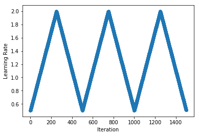
+As an example, we implement the triangular cyclical schedule presented in ["Cyclical Learning Rates for Training Neural Networks" by Leslie N. Smith (2015)](https://arxiv.org/abs/1506.01186). We use slightly different terminology to the paper here because we use `cycle_length` that is twice the 'stepsize' used in the paper. We repeat cycles, each with a length of 500 iterations and lower and upper learning rate bounds of 0.5 and 2 respectively.
+
+
+```python
+schedule = CyclicalSchedule(TriangularSchedule, min_lr=0.5, max_lr=2, cycle_length=500)
+plot_schedule(schedule)
+```
+
+
+ <!--notebook-skip-line-->
+
+
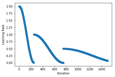
+And lastly, we implement the scheduled used in ["SGDR: Stochastic Gradient Descent with Warm Restarts" by Ilya Loshchilov, Frank Hutter (2016)](https://arxiv.org/abs/1608.03983). We repeat cosine annealing schedules, but each time we halve the magnitude and double the cycle length.
+
+
+```python
+schedule = CyclicalSchedule(CosineAnnealingSchedule, min_lr=0.01, max_lr=2,
+ cycle_length=250, cycle_length_decay=2, cycle_magnitude_decay=0.5)
+plot_schedule(schedule)
+```
+
+
+ <!--notebook-skip-line-->
+
+
+**_Want to learn more?_** Checkout the "Learning Rate Schedules" tutorial for a more basic overview of learning rates found in `mx.lr_scheduler`, and an example of how to use them while training your own models.
+
+<!-- INSERT SOURCE DOWNLOAD BUTTONS -->
\ No newline at end of file
diff --git a/docs/tutorials/index.md b/docs/tutorials/index.md
index 39a5aa4..9084e14 100644
--- a/docs/tutorials/index.md
+++ b/docs/tutorials/index.md
@@ -42,6 +42,8 @@ Select API:
* [Inference using an ONNX model](/tutorials/onnx/inference_on_onnx_model.html)
* [Fine-tuning an ONNX model on Gluon](/tutorials/onnx/fine_tuning_gluon.html)
* [Visualizing Decisions of Convolutional Neural Networks](/tutorials/vision/cnn_visualization.html)
+ * [Learning Rate Schedules](/tutorials/gluon/learning_rate_schedules.html)
+ * [Advanced Learning Rate Schedules](/tutorials/gluon/learning_rate_schedules_advanced.html)
* [Profiling MXNet Models](/tutorials/python/profiler.html)
* API Guides
* Core APIs
diff --git a/tests/tutorials/test_tutorials.py b/tests/tutorials/test_tutorials.py
index 4741df5..44cbeff 100644
--- a/tests/tutorials/test_tutorials.py
+++ b/tests/tutorials/test_tutorials.py
@@ -156,7 +156,13 @@ def test_gluon_hybrid():
def test_gluon_pretrained_models():
assert _test_tutorial_nb('gluon/pretrained_models')
+
+def test_gluon_learning_rate_schedules():
+ assert _test_tutorial_nb('gluon/learning_rate_schedules')
+def test_gluon_learning_rate_schedules_advanced():
+ assert _test_tutorial_nb('gluon/learning_rate_schedules_advanced')
+
def test_nlp_cnn():
assert _test_tutorial_nb('nlp/cnn')
@@ -193,6 +199,9 @@ def test_python_kvstore():
def test_python_types_of_data_augmentation():
assert _test_tutorial_nb('python/types_of_data_augmentation')
+def test_python_profiler():
+ assert _test_tutorial_nb('python/profiler')
+
def test_sparse_row_sparse():
assert _test_tutorial_nb('sparse/row_sparse')
@@ -212,7 +221,4 @@ def test_vision_large_scale_classification():
assert _test_tutorial_nb('vision/large_scale_classification')
def test_vision_cnn_visualization():
- assert _test_tutorial_nb('vision/cnn_visualization')
-
-def test_python_profiler():
- assert _test_tutorial_nb('python/profiler')
+ assert _test_tutorial_nb('vision/cnn_visualization')
\ No newline at end of file