[GitHub] thomelane commented on a change in pull request #11296: Adding 2 tutorials on Learning Rate Schedules

[GitBox <gi...@apache.org>]

thomelane commented on a change in pull request #11296: Adding 2 tutorials on Learning Rate Schedules
URL: https://github.com/apache/incubator-mxnet/pull/11296#discussion_r196613954
 
 

 ##########
 File path: docs/tutorials/gluon/learning_rate_schedules_advanced.md
 ##########
 @@ -0,0 +1,308 @@
+
+ # Advanced Learning Rate Schedules
+
+Given the importance of learning rate and the learning rate schedule for training neural networks, there have been a number of research papers published recently on the subject. Although many practitioners are using simple learning rate schedules such as stepwise decay, research has shown that there are other strategies that work better in most situations. We implement a number of different schedule shapes in this tutorial and introduce cyclical schedules.
+
+See the "Learning Rate Schedules" tutorial for a more basic overview of learning rates, and an example of how to use them while training your own models.
+
+
+```python
+%matplotlib inline
+import copy
+import math
+import mxnet as mx
+import numpy as np
+import matplotlib.pyplot as plt
+```
+
+
+```python
+def plot_schedule(schedule_fn, iterations=1500):
+    iterations = [i for i in range(iterations)]
+    lrs = [schedule_fn(i) for i in iterations]
+    plt.scatter(iterations, lrs)
+    plt.xlabel("Iteration")
+    plt.ylabel("Learning Rate")
+    plt.show()
+```
+
+## Custom Schedule Shapes
+
+### (Slanted) Triangular
+
+While trying to push the boundaries of batch size for faster training, [Priya Goyal et al. (2017)](https://arxiv.org/abs/1706.02677) found that having a smooth linear warm up in the learning rate at the start of training improved the stability of the optimizer and lead to better solutions. It was found that a smooth increases gave improved performance over stepwise increases.
+
+We look at "warm-up" in more detail later in the tutorial, but this could be viewed as a specific case of the **"triangular"** schedule that was proposed by [Leslie N. Smith (2015)](https://arxiv.org/abs/1506.01186). Quite simply, the schedule linearly increases then decreases between a lower and upper bound. Originally it was suggested this schedule be used as part of a cyclical schedule but more recently researchers have been using a single cycle.
+
+One adjustment proposed by [Jeremy Howard, Sebastian Ruder (2018)](https://arxiv.org/abs/1801.06146) was to change the ratio between the increasing and decreasing stages, instead of the 50:50 split. Changing the increasing fraction (`inc_fraction!=0.5`) leads to a **"slanted triangular"** schedule. Using `inc_fraction<0.5` tends to give better results.
+
+
+```python
+class TriangularSchedule():
+    def __init__(self, min_lr, max_lr, cycle_length, inc_fraction=0.5):     
+        """
+        min_lr: lower bound for learning rate (float)
+        max_lr: upper bound for learning rate (float)
+        cycle_length: iterations between start and finish (int)
+        inc_fraction: fraction of iterations spent in increasing stage (float)
+        """
+        self.min_lr = min_lr
+        self.max_lr = max_lr
+        self.cycle_length = cycle_length
+        self.inc_fraction = inc_fraction
+        
+    def __call__(self, iteration):
+        if iteration <= self.cycle_length*self.inc_fraction:
+            unit_cycle = iteration * 1/(self.cycle_length*self.inc_fraction)
+        elif iteration <= self.cycle_length:
+            unit_cycle = (self.cycle_length - iteration) * 1/(self.cycle_length*(1-self.inc_fraction))
+        else:
+            unit_cycle = 0
+        adjusted_cycle = (unit_cycle * (self.max_lr - self.min_lr)) + self.min_lr
+        return adjusted_cycle
+```
+
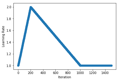
+We look an example of a slanted triangular schedule that increases from a learning rate of 1 to 2, and back to 1 over 1000 iterations. Since we set `inc_fraction=0.2`, 200 iterations are used for the increasing stage, and 800 for the decreasing stage. After this, the schedule stays at the lower bound indefinitely.
+
+
+```python
+schedule = TriangularSchedule(min_lr=1, max_lr=2, cycle_length=1000, inc_fraction=0.2)
+plot_schedule(schedule)
+```
+
+
+![png](https://raw.githubusercontent.com/dmlc/web-data/master/mxnet/doc/tutorials/lr_schedules/adv_triangular.png) <!--notebook-skip-line-->
+
+
+### Cosine
+
+Continuing with the idea that smooth decay profiles give improved performance over stepwise decay, [Ilya Loshchilov, Frank Hutter (2016)](https://arxiv.org/abs/1608.03983) used **"cosine annealing"** schedules to good effect. As with triangular schedules, the original idea was that this should be used as part of a cyclical schedule, but we begin by implementing the cosine annealing component before the full Stochastic Gradient Descent with Warm Restarts (SGDR) method later in the tutorial.
+
+
+```python
+class CosineAnnealingSchedule():
+    def __init__(self, min_lr, max_lr, cycle_length):
+        """
+        min_lr: lower bound for learning rate (float)
+        max_lr: upper bound for learning rate (float)
+        cycle_length: iterations between start and finish (int)
+        """
+        self.min_lr = min_lr
+        self.max_lr = max_lr
+        self.cycle_length = cycle_length
+        
+    def __call__(self, iteration):
+        if iteration <= self.cycle_length:
+            unit_cycle = (1 + math.cos(iteration*math.pi/self.cycle_length))/2
+            adjusted_cycle = (unit_cycle * (self.max_lr - self.min_lr)) + self.min_lr
+            return adjusted_cycle
+        else:
+            return self.min_lr
+```
+
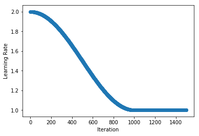
+We look at an example of a cosine annealing schedule that smoothing decreases from a learning rate of 2 to 1 across 1000 iterations. After this, the schedule stays at the lower bound indefinietly.
+
+
+```python
+schedule = CosineAnnealingSchedule(min_lr=1, max_lr=2, cycle_length=1000)
+plot_schedule(schedule)
+```
+
+
+![png](https://raw.githubusercontent.com/dmlc/web-data/master/mxnet/doc/tutorials/lr_schedules/adv_cosine.png) <!--notebook-skip-line-->
+
+
+## Custom Schedule Modifiers
+
+We now take a look some adjustments that can be made to existing schedules. We see how to add linear warm-up and its compliment linear cool-down, before using this to implement the "1-Cycle" schedule used by [Leslie N. Smith, Nicholay Topin (2017)](https://arxiv.org/abs/1708.07120) for "super-convergence". We then look at cyclical schedules and implement the original cyclical schedule from [Leslie N. Smith (2015)](https://arxiv.org/abs/1506.01186) before finishing with a look at ["SGDR: Stochastic Gradient Descent with Warm Restarts" by Ilya Loshchilov, Frank Hutter (2016)](https://arxiv.org/abs/1608.03983).
+
+Unlike the schedules above and those implemented in `mx.lr_scheduler`, these classes are designed to modify existing schedules so they take the argument `schedule` (for initialized schedules) or `schedule_class` when being initialized.
+
+### Warm-Up
+
+Using the idea of linear warm-up of the learning rate proposed in ["Accurate, Large Minibatch SGD: Training ImageNet in 1 Hour" by Priya Goyal et al. (2017)](https://arxiv.org/abs/1706.02677), we implement a wrapper class that adds warm-up to an existing schedule. Going from `start_lr` to the initial learning rate of the `schedule` over `length` iterations, this adjustment is useful when training with large batch sizes.
+
+
+```python
+class LinearWarmUp():
+    def __init__(self, schedule, start_lr, length):
+        """
+        schedule: a pre-initialized schedule (e.g. TriangularSchedule(min_lr=0.5, max_lr=2, cycle_length=500))
+        start_lr: learning rate used at start of the warm-up (float)
+        length: number of iterations used for the warm-up (int)
+        """
+        self.schedule = schedule
+        self.start_lr = start_lr
+        # calling mx.lr_scheduler.LRScheduler effects state, so calling a copy
+        self.finish_lr = copy.copy(schedule)(0)
+        self.length = length
+    
+    def __call__(self, iteration):
+        if iteration <= self.length:
+            return iteration * (self.finish_lr-self.start_lr)/(self.length) + self.start_lr
+        else:
+            return self.schedule(iteration - self.length)
+```
+
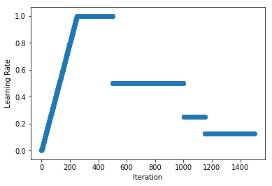
+As an example, we add a linear warm-up of the learning rate (from 0 to 1 over 250 iterations) to a stepwise decay schedule. We first create the `MultiFactorScheduler` (and set the `base_lr`) and then pass it to `LinearWarmUp` to add the warm-up at the start. We can use `LinearWarmUp` with any other schedule including `CosineAnnealingSchedule`.
+
+
+```python
+schedule = mx.lr_scheduler.MultiFactorScheduler(step=[250, 750, 900], factor=0.5)
+schedule.base_lr = 1
+schedule = LinearWarmUp(schedule, start_lr=0, length=250)
+plot_schedule(schedule)
+```
+
+
+![png](https://raw.githubusercontent.com/dmlc/web-data/master/mxnet/doc/tutorials/lr_schedules/adv_warmup.png) <!--notebook-skip-line-->
+
+
+### Cool-Down
+
+Similarly, we could add a linear cool-down period to our schedule and this is used in the "1-Cycle" schedule proposed by [Leslie N. Smith, Nicholay Topin (2017)](https://arxiv.org/abs/1708.07120) to train neural networks very quickly in certain circumstances (coined "super-convergence"). We reduce the learning rate from its value at `start_idx` of `schedule` to `finish_lr` over a period of `length`, and then maintain `finish_lr` thereafter.
+
+
+```python
+class LinearCoolDown():
+    def __init__(self, schedule, finish_lr, start_idx, length):
+        """
+        schedule: a pre-initialized schedule (e.g. TriangularSchedule(min_lr=0.5, max_lr=2, cycle_length=500))
+        finish_lr: learning rate used at end of the cool-down (float)
+        start_idx: iteration to start the cool-down (int)
+        length: number of iterations used for the cool-down (int)
+        """
+        self.schedule = schedule
+        # calling mx.lr_scheduler.LRScheduler effects state, so calling a copy
+        self.start_lr = copy.copy(self.schedule)(start_idx)
+        self.finish_lr = finish_lr
+        self.start_idx = start_idx
+        self.finish_idx = start_idx + length
+        self.length = length
+    
+    def __call__(self, iteration):
+        if iteration <= self.start_idx:
+            return self.schedule(iteration)
+        elif iteration <= self.finish_idx:
+            return (iteration - self.start_idx) * (self.finish_lr-self.start_lr)/(self.length) + self.start_lr
+        else:
+            return self.finish_lr
+```
+
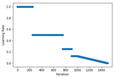
+As an example, we apply learning rate cool-down to a `MultiFactorScheduler`. Starting the cool-down at iteration 1000, we reduce the learning rate linearly from 0.125 to 0.001 over 500 iterations, and hold the learning rate at 0.001 after this.
+
+
+```python
+schedule = mx.lr_scheduler.MultiFactorScheduler(step=[250, 750, 900], factor=0.5)
+schedule.base_lr = 1
+schedule = LinearCoolDown(schedule, finish_lr=0.001, start_idx=1000, length=500)
+plot_schedule(schedule)
+```
+
+
+![png](https://raw.githubusercontent.com/dmlc/web-data/master/mxnet/doc/tutorials/lr_schedules/adv_cooldown.png) <!--notebook-skip-line-->
+
+
+#### 1-Cycle: for "Super-Convergence"
+
+Cool-down is used in the "1-Cycle" schedule proposed by [Leslie N. Smith, Nicholay Topin (2017)](https://arxiv.org/abs/1708.07120) to train neural networks very quickly in certain circumstances (coined "super-convergence"). We implement a single and symmetric cycle of the triangular schedule above (i.e. `inc_fraction=0.5`), followed by a cool-down period of `cooldown_length` iterations.
 
 Review comment:
   Agreed, removed.

----------------------------------------------------------------
This is an automated message from the Apache Git Service.
To respond to the message, please log on GitHub and use the
URL above to go to the specific comment.
 
For queries about this service, please contact Infrastructure at:
users@infra.apache.org


With regards,
Apache Git Services