[GitHub] thomelane commented on a change in pull request #11304: Added Learning Rate Finder tutorial

[GitBox <gi...@apache.org>]

thomelane commented on a change in pull request #11304: Added Learning Rate Finder tutorial
URL: https://github.com/apache/incubator-mxnet/pull/11304#discussion_r197568683
 
 

 ##########
 File path: docs/tutorials/gluon/learning_rate_finder.md
 ##########
 @@ -0,0 +1,321 @@
+
+# Learning Rate Finder
+
+Setting the learning rate for stochastic gradient descent (SGD) is crucially important when training neural network because it controls both the speed of convergence and the ultimate performance of the network. Set the learning too low and you could be twiddling your thumbs for quite some time as the parameters update very slowly. Set it too high and the updates will skip over optimal solutions, or worse the optimizer might not converge at all!
+
+Leslie Smith from the U.S. Naval Research Laboratory presented a method for finding a good learning rate in a paper called ["Cyclical Learning Rates for Training Neural Networks"](https://arxiv.org/abs/1506.01186). We take a look at the central idea of the paper, cyclical learning rate schedules, in the tutorial found here, but in this tutorial we implement a 'Learning Rate Finder' in MXNet with the Gluon API that you can use while training your own networks.
+
+## Simple Idea
+
+Given an initialized network, a defined loss and a training dataset we take the following steps:
+
+1. train one batch at a time (a.k.a. an iteration)
+2. start with a very small learning rate (e.g. 0.000001) and slowly increase it every iteration
+3. record the training loss and continue until we see the training loss diverge
+
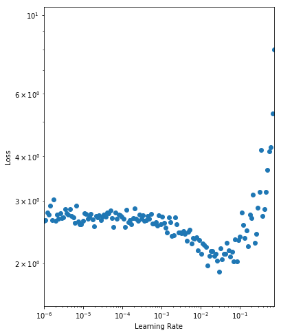
+We then analyse the results by plotting a graph of the learning rate against the training loss as seen below (taking note of the log scales).
+
+![png](https://raw.githubusercontent.com/dmlc/web-data/master/mxnet/doc/tutorials/lr_finder/finder_plot.png) <!--notebook-skip-line-->
+
+As expected, for very small learning rates we don't see much change in the loss as the paramater updates are negligible. At a learning rate of 0.001 we start to see the loss fall. Setting the initial learning rate here is reasonable, but we still have the potential to learn faster. We observe a drop in the loss up until 0.1 where the loss appears to diverge. We want to set the initial learning rate as high as possible before the loss becomes unstable, so we choose a learning rate of 0.05.
+
+## Epoch to Iteration
+
+Usually our unit of work is an epoch (a full pass through the dataset) and the learning rate would typically be held constant throughout the epoch. With the Learning Rate Finder (and cyclical learning rate schedules) we are required to vary the learning rate every iteration. As such we structure our training code so that a single iteration can be run with a given learning rate. You can implement Learner as you wish. Just initialize the network, define the loss and trainer in `__init__` and keep your training logic for a single batch in `iteration`.
+
+
+```python
+import mxnet as mx
+
+# Set seed for reproducibility
+mx.random.seed(42)
+
+class Learner():
+    def __init__(self, net, data_loader, ctx):
+        """
+        net: network (mx.gluon.Block)
+        data_loader: training data loader (mx.gluon.data.DataLoader)
+        ctx: context (mx.gpu or mx.cpu)
+        """
+        self.net = net
+        self.data_loader = data_loader
+        self.ctx = ctx
+        # So we don't need to be in `for batch in data_loader` scope
+        # and can call for next batch in `iteration`
+        self.data_loader_iter = iter(self.data_loader)
+        self.net.collect_params().initialize(mx.init.Xavier(), ctx=self.ctx)
+        self.loss_fn = mx.gluon.loss.SoftmaxCrossEntropyLoss()
+        self.trainer = mx.gluon.Trainer(net.collect_params(), 'sgd', {'learning_rate': .001})
+        
+    def iteration(self, lr=None, take_step=True):
+        """
+        lr: learning rate to use for iteration (float)
+        take_step: take trainer step to update weights (boolean)
+        """
+        # Update learning rate if different this iteration
+        if lr and (lr != self.trainer.learning_rate):
+            self.trainer.set_learning_rate(lr)
+        # Get next batch, and move context (e.g. to GPU if set)
+        data, label = next(self.data_loader_iter)
+        data = data.as_in_context(self.ctx)
+        label = label.as_in_context(self.ctx)
+        # Standard forward and backward pass
+        with mx.autograd.record():
+            output = self.net(data)
+            loss = self.loss_fn(output, label)
+        loss.backward()     
+        # Update parameters
+        if take_step: self.trainer.step(data.shape[0])  
+        # Set and return loss.
+        # Although notice this is still an MXNet NDArray to avoid blocking
+        self.iteration_loss = mx.nd.mean(loss)
+        return self.iteration_loss
+
+    def close(self):
+        # Close open iterator and associated workers
+        self.data_loader_iter.shutdown()
+```
+
+We also adjust our `DataLoader` so that it continuously provides batches of data and doesn't stop after a single epoch. We can then call `iteration` as many times as required for the loss to diverge as part of the Learning Rate Finder process. We implement a custom `BatchSampler` for this, that keeps returning random indices of samples to be included in the next batch. We use the CIFAR-10 dataset for image classification to test our Learning Rate Finder.
+
+
+```python
+from multiprocessing import cpu_count
+from mxnet.gluon.data.vision import transforms
+
+transform = transforms.Compose([
+    # Switches HWC to CHW, and converts to `float32`
+    transforms.ToTensor(),
+    # Channel-wise, using pre-computed means and stds 
+    transforms.Normalize(mean=[0.4914, 0.4822, 0.4465],
+                         std=[0.2023, 0.1994, 0.2010])
+])
+
+dataset = mx.gluon.data.vision.datasets.CIFAR10(train=True).transform_first(transform)
+
+class ContinuousBatchSampler():
+    def __init__(self, sampler, batch_size):
+        self._sampler = sampler
+        self._batch_size = batch_size
+
+    def __iter__(self):
+        batch = []
+        while True:
+            for i in self._sampler:
+                batch.append(i)
+                if len(batch) == self._batch_size:
+                    yield batch
+                    batch = []
+
+sampler = mx.gluon.data.RandomSampler(len(dataset))
+batch_sampler = ContinuousBatchSampler(sampler, batch_size=128)
+data_loader = mx.gluon.data.DataLoader(dataset, batch_sampler=batch_sampler, num_workers=cpu_count())
+```
+
+## Implementation
+
+With preparation complete, we're ready to write our Learning Rate Finder that wraps the `Learner` we defined above. We implement a `find` method for the procedure, and `plot` for the visualization. Starting with a very low learning rate as defined by `lr_start` we train one iteration at a time and keep multiplying the learning rate by `lr_multiplier`. We analyse the loss and continue until it diverges according to `LRFinderStoppingCriteria` (which is defined later on). You may also notice that we save the parameters and state of the optimizer before the process and restore afterwards. This is so the Learning Rate Finder process doesn't impact the state of the model, and can be used at any point during training.
 
 Review comment:
   Same as above.

----------------------------------------------------------------
This is an automated message from the Apache Git Service.
To respond to the message, please log on GitHub and use the
URL above to go to the specific comment.
 
For queries about this service, please contact Infrastructure at:
users@infra.apache.org


With regards,
Apache Git Services