You are viewing a plain text version of this content. The canonical link for it is here.
Posted to commits@mxnet.apache.org by la...@apache.org on 2020/12/08 16:14:25 UTC
[incubator-mxnet] branch master updated: [DOC] Fix warnings in
tutorials and turn on -W (#19624)
This is an automated email from the ASF dual-hosted git repository.
lausen pushed a commit to branch master
in repository https://gitbox.apache.org/repos/asf/incubator-mxnet.git
The following commit(s) were added to refs/heads/master by this push:
new 6cbd3ae [DOC] Fix warnings in tutorials and turn on -W (#19624)
6cbd3ae is described below
commit 6cbd3ae772550d3e61c455590cea29373362af02
Author: Sheng Zha <sz...@users.noreply.github.com>
AuthorDate: Tue Dec 8 11:13:09 2020 -0500
[DOC] Fix warnings in tutorials and turn on -W (#19624)
---
ci/docker/runtime_functions.sh | 40 +-
.../normalization/imgs => _static}/NCHW_BN.png | Bin
.../normalization/imgs => _static}/NCHW_IN.png | Bin
.../normalization/imgs => _static}/NCHW_LN.png | Bin
.../normalization/imgs => _static}/NTC_BN.png | Bin
.../normalization/imgs => _static}/NTC_IN.png | Bin
.../normalization/imgs => _static}/NTC_LN.png | Bin
docs/python_docs/_static/autograd_gradient.png | Bin 0 -> 39559 bytes
.../packages/gluon/blocks => _static}/blocks.svg | 0
.../loss/images => _static}/contrastive_loss.jpeg | Bin
.../packages/gluon/loss => _static}/ctc_loss.png | Bin
.../imgs => _static}/data_normalization.jpeg | Bin
.../blocks/activations/images => _static}/elu.png | Bin
.../blocks/activations/images => _static}/gelu.png | Bin
.../gluon/loss/images => _static}/inuktitut_1.png | Bin
.../gluon/loss/images => _static}/inuktitut_2.png | Bin
.../activations/images => _static}/leakyrelu.png | Bin
.../activations/images => _static}/prelu.png | Bin
.../blocks/activations/images => _static}/relu.png | Bin
.../blocks/activations/images => _static}/selu.png | Bin
.../activations/images => _static}/sigmoid.png | Bin
.../blocks/activations/images => _static}/silu.png | Bin
.../activations/images => _static}/softrelu.png | Bin
.../activations/images => _static}/softsign.png | Bin
.../activations/images => _static}/swish.png | Bin
.../blocks/activations/images => _static}/tanh.png | Bin
.../gluon/loss => _static}/triplet_loss.png | Bin
docs/python_docs/python/Makefile_sphinx | 2 +-
docs/python_docs/python/api/gluon/rnn/index.rst | 1 -
docs/python_docs/python/api/kvstore/index.rst | 35 +-
docs/python_docs/python/api/npx/index.rst | 1 +
.../python/tutorials/deploy/export/onnx.md | 12 +-
.../getting-started/crash-course/0-introduction.md | 12 +-
.../getting-started/crash-course/1-nparray.md | 50 +-
.../getting-started/crash-course/2-create-nn.md | 1134 +++++++++++---------
.../getting-started/crash-course/3-autograd.md | 48 +-
.../getting-started/crash-course/4-components.md | 79 +-
.../getting-started/crash-course/5-datasets.md | 98 +-
.../getting-started/crash-course/6-train-nn.md | 106 +-
.../getting-started/crash-course/7-use-gpus.md | 35 +-
.../gluon_from_experiment_to_deployment.md | 19 +-
.../logistic_regression_explained.md | 20 +-
.../tutorials/getting-started/to-mxnet/pytorch.md | 18 +-
.../python/tutorials/packages/autograd/index.md | 12 +-
.../gluon/blocks/activations/activations.md | 48 +-
.../packages/gluon/blocks/custom-layer.md | 2 +-
.../gluon/blocks/custom_layer_beginners.md | 2 +-
.../tutorials/packages/gluon/blocks/hybridize.md | 8 +-
.../python/tutorials/packages/gluon/blocks/init.md | 6 +-
.../python/tutorials/packages/gluon/blocks/nn.md | 32 +-
.../tutorials/packages/gluon/blocks/parameters.md | 22 +-
.../packages/gluon/blocks/save_load_params.md | 10 +-
.../packages/gluon/data/data_augmentation.md | 34 +-
.../tutorials/packages/gluon/data/datasets.md | 32 +-
.../tutorials/packages/gluon/image/info_gan.md | 68 +-
.../python/tutorials/packages/gluon/image/mnist.md | 22 +-
.../tutorials/packages/gluon/loss/custom-loss.md | 14 +-
.../tutorials/packages/gluon/loss/kl_divergence.md | 16 +-
.../python/tutorials/packages/gluon/loss/loss.md | 34 +-
.../packages/gluon/training/fit_api_tutorial.md | 10 +-
.../learning_rates/learning_rate_finder.md | 4 +-
.../learning_rates/learning_rate_schedules.md | 14 +-
.../learning_rate_schedules_advanced.md | 14 +-
.../packages/gluon/training/normalization/index.md | 18 +-
.../tutorials/packages/gluon/training/trainer.md | 24 +-
.../python/tutorials/packages/kvstore/kvstore.md | 2 +-
.../packages/legacy/ndarray/01-ndarray-intro.md | 6 +-
.../legacy/ndarray/02-ndarray-operations.md | 2 +-
.../packages/legacy/ndarray/03-ndarray-contexts.md | 4 +-
.../legacy/ndarray/gotchas_numpy_in_mxnet.md | 20 +-
.../packages/legacy/ndarray/sparse/csr.md | 12 +-
.../packages/legacy/ndarray/sparse/row_sparse.md | 12 +-
.../packages/legacy/ndarray/sparse/train_gluon.md | 74 +-
.../python/tutorials/packages/np/index.rst | 4 +-
.../python/tutorials/packages/np/np-vs-numpy.md | 18 +-
.../tutorials/packages/onnx/fine_tuning_gluon.md | 8 +-
.../packages/onnx/inference_on_onnx_model.md | 21 +-
.../python/tutorials/packages/optimizer/index.md | 61 +-
.../tutorials/performance/backend/profiler.md | 14 +-
python/mxnet/gluon/rnn/rnn_cell.py | 6 +-
python/mxnet/numpy/random.py | 70 +-
src/operator/contrib/transformer.cc | 86 +-
82 files changed, 1333 insertions(+), 1243 deletions(-)
diff --git a/ci/docker/runtime_functions.sh b/ci/docker/runtime_functions.sh
index be8cdfb..53330bc 100755
--- a/ci/docker/runtime_functions.sh
+++ b/ci/docker/runtime_functions.sh
@@ -712,6 +712,7 @@ sanity_cpp() {
sanity_python() {
set -ex
+ export DMLC_LOG_STACK_TRACE_DEPTH=100
python3 -m pylint --rcfile=ci/other/pylintrc --ignore-patterns=".*\.so$$,.*\.dll$$,.*\.dylib$$" python/mxnet
OMP_NUM_THREADS=$(expr $(nproc) / 4) pytest -n 4 tests/tutorials/test_sanity_tutorials.py
}
@@ -728,7 +729,7 @@ cd_unittest_ubuntu() {
export MXNET_SUBGRAPH_VERBOSE=0
export MXNET_ENABLE_CYTHON=0
export CD_JOB=1 # signal this is a CD run so any unecessary tests can be skipped
- export DMLC_LOG_STACK_TRACE_DEPTH=10
+ export DMLC_LOG_STACK_TRACE_DEPTH=100
local mxnet_variant=${1:?"This function requires a mxnet variant as the first argument"}
@@ -767,7 +768,7 @@ unittest_ubuntu_python3_cpu() {
export MXNET_STORAGE_FALLBACK_LOG_VERBOSE=0
export MXNET_SUBGRAPH_VERBOSE=0
export MXNET_ENABLE_CYTHON=0
- export DMLC_LOG_STACK_TRACE_DEPTH=10
+ export DMLC_LOG_STACK_TRACE_DEPTH=100
OMP_NUM_THREADS=$(expr $(nproc) / 4) pytest -m 'not serial' -k 'not test_operator' -n 4 --durations=50 --cov-report xml:tests_unittest.xml --verbose tests/python/unittest
MXNET_ENGINE_TYPE=NaiveEngine \
OMP_NUM_THREADS=$(expr $(nproc) / 4) pytest -m 'not serial' -k 'test_operator' -n 4 --durations=50 --cov-report xml:tests_unittest.xml --cov-append --verbose tests/python/unittest
@@ -781,7 +782,7 @@ unittest_ubuntu_python3_cpu_mkldnn() {
export MXNET_STORAGE_FALLBACK_LOG_VERBOSE=0
export MXNET_SUBGRAPH_VERBOSE=0
export MXNET_ENABLE_CYTHON=0
- export DMLC_LOG_STACK_TRACE_DEPTH=10
+ export DMLC_LOG_STACK_TRACE_DEPTH=100
OMP_NUM_THREADS=$(expr $(nproc) / 4) pytest -m 'not serial' -k 'not test_operator' -n 4 --durations=50 --cov-report xml:tests_unittest.xml --verbose tests/python/unittest
MXNET_ENGINE_TYPE=NaiveEngine \
OMP_NUM_THREADS=$(expr $(nproc) / 4) pytest -m 'not serial' -k 'test_operator' -n 4 --durations=50 --cov-report xml:tests_unittest.xml --cov-append --verbose tests/python/unittest
@@ -797,7 +798,7 @@ unittest_ubuntu_python3_gpu() {
export MXNET_SUBGRAPH_VERBOSE=0
export CUDNN_VERSION=${CUDNN_VERSION:-7.0.3}
export MXNET_ENABLE_CYTHON=0
- export DMLC_LOG_STACK_TRACE_DEPTH=10
+ export DMLC_LOG_STACK_TRACE_DEPTH=100
MXNET_GPU_MEM_POOL_TYPE=Unpooled \
OMP_NUM_THREADS=$(expr $(nproc) / 4) pytest -m 'not serial' -k 'not test_operator and not test_amp_init.py' -n 4 --durations=50 --cov-report xml:tests_gpu.xml --verbose tests/python/gpu
MXNET_GPU_MEM_POOL_TYPE=Unpooled \
@@ -816,7 +817,7 @@ unittest_ubuntu_python3_gpu_cython() {
export CUDNN_VERSION=${CUDNN_VERSION:-7.0.3}
export MXNET_ENABLE_CYTHON=1
export MXNET_ENFORCE_CYTHON=1
- export DMLC_LOG_STACK_TRACE_DEPTH=10
+ export DMLC_LOG_STACK_TRACE_DEPTH=100
check_cython
MXNET_GPU_MEM_POOL_TYPE=Unpooled \
OMP_NUM_THREADS=$(expr $(nproc) / 4) pytest -m 'not serial' -k 'not test_operator and not test_amp_init.py' -n 4 --durations=50 --cov-report xml:tests_gpu.xml --verbose tests/python/gpu
@@ -834,7 +835,7 @@ unittest_ubuntu_python3_gpu_nocudnn() {
export MXNET_SUBGRAPH_VERBOSE=0
export CUDNN_OFF_TEST_ONLY=true
export MXNET_ENABLE_CYTHON=0
- export DMLC_LOG_STACK_TRACE_DEPTH=10
+ export DMLC_LOG_STACK_TRACE_DEPTH=100
MXNET_GPU_MEM_POOL_TYPE=Unpooled \
OMP_NUM_THREADS=$(expr $(nproc) / 4) pytest -m 'not serial' -k 'not test_operator and not test_amp_init.py' -n 4 --durations=50 --cov-report xml:tests_gpu.xml --verbose tests/python/gpu
MXNET_GPU_MEM_POOL_TYPE=Unpooled \
@@ -846,6 +847,7 @@ unittest_ubuntu_python3_gpu_nocudnn() {
unittest_cpp() {
set -ex
+ export DMLC_LOG_STACK_TRACE_DEPTH=100
build/tests/mxnet_unit_tests
}
@@ -853,6 +855,7 @@ unittest_centos7_cpu() {
set -ex
source /opt/rh/rh-python36/enable
cd /work/mxnet
+ export DMLC_LOG_STACK_TRACE_DEPTH=100
OMP_NUM_THREADS=$(expr $(nproc) / 4) python -m pytest -m 'not serial' -k 'not test_operator' -n 4 --durations=50 --cov-report xml:tests_unittest.xml --verbose tests/python/unittest
MXNET_ENGINE_TYPE=NaiveEngine \
OMP_NUM_THREADS=$(expr $(nproc) / 4) python -m pytest -m 'not serial' -k 'test_operator' -n 4 --durations=50 --cov-report xml:tests_unittest.xml --cov-append --verbose tests/python/unittest
@@ -865,7 +868,7 @@ unittest_centos7_gpu() {
source /opt/rh/rh-python36/enable
cd /work/mxnet
export CUDNN_VERSION=${CUDNN_VERSION:-7.0.3}
- export DMLC_LOG_STACK_TRACE_DEPTH=10
+ export DMLC_LOG_STACK_TRACE_DEPTH=100
MXNET_GPU_MEM_POOL_TYPE=Unpooled \
OMP_NUM_THREADS=$(expr $(nproc) / 4) pytest -m 'not serial' -k 'not test_operator and not test_amp_init.py' -n 4 --durations=50 --cov-report xml:tests_gpu.xml --cov-append --verbose tests/python/gpu
MXNET_GPU_MEM_POOL_TYPE=Unpooled \
@@ -879,7 +882,7 @@ integrationtest_ubuntu_cpu_onnx() {
set -ex
export PYTHONPATH=./python/
export MXNET_SUBGRAPH_VERBOSE=0
- export DMLC_LOG_STACK_TRACE_DEPTH=10
+ export DMLC_LOG_STACK_TRACE_DEPTH=100
python3 tests/python/unittest/onnx/backend_test.py
OMP_NUM_THREADS=$(expr $(nproc) / 4) pytest -n 4 tests/python/unittest/onnx/mxnet_export_test.py
OMP_NUM_THREADS=$(expr $(nproc) / 4) pytest -n 4 tests/python/unittest/onnx/test_models.py
@@ -894,7 +897,7 @@ integrationtest_ubuntu_cpu_dist_kvstore() {
export MXNET_STORAGE_FALLBACK_LOG_VERBOSE=0
export MXNET_SUBGRAPH_VERBOSE=0
export MXNET_USE_OPERATOR_TUNING=0
- export DMLC_LOG_STACK_TRACE_DEPTH=10
+ export DMLC_LOG_STACK_TRACE_DEPTH=100
cd tests/nightly/
python3 ../../tools/launch.py -n 7 --launcher local python3 dist_sync_kvstore.py --type=gluon_step_cpu
python3 ../../tools/launch.py -n 7 --launcher local python3 dist_sync_kvstore.py --type=gluon_sparse_step_cpu
@@ -910,6 +913,7 @@ integrationtest_ubuntu_cpu_dist_kvstore() {
integrationtest_ubuntu_gpu_dist_kvstore() {
set -ex
+ export DMLC_LOG_STACK_TRACE_DEPTH=100
pushd .
cd /work/mxnet/python
pip3 install -e .
@@ -929,7 +933,7 @@ integrationtest_ubuntu_gpu_byteps() {
git clone -b v0.2.3 https://github.com/bytedance/byteps ~/byteps
export MXNET_STORAGE_FALLBACK_LOG_VERBOSE=0
export MXNET_SUBGRAPH_VERBOSE=0
- export DMLC_LOG_STACK_TRACE_DEPTH=10
+ export DMLC_LOG_STACK_TRACE_DEPTH=100
cd tests/nightly/
export NVIDIA_VISIBLE_DEVICES=0
@@ -952,7 +956,7 @@ test_ubuntu_cpu_python3() {
set -ex
pushd .
export MXNET_LIBRARY_PATH=/work/build/libmxnet.so
- export DMLC_LOG_STACK_TRACE_DEPTH=10
+ export DMLC_LOG_STACK_TRACE_DEPTH=100
VENV=mxnet_py3_venv
virtualenv -p `which python3` $VENV
source $VENV/bin/activate
@@ -976,7 +980,7 @@ unittest_ubuntu_python3_arm() {
export MXNET_STORAGE_FALLBACK_LOG_VERBOSE=0
export MXNET_SUBGRAPH_VERBOSE=0
export MXNET_ENABLE_CYTHON=0
- export DMLC_LOG_STACK_TRACE_DEPTH=10
+ export DMLC_LOG_STACK_TRACE_DEPTH=100
python3 -m pytest -n 2 --verbose tests/python/unittest/test_engine.py
}
@@ -1010,7 +1014,7 @@ test_rat_check() {
nightly_test_KVStore_singleNode() {
set -ex
export PYTHONPATH=./python/
- export DMLC_LOG_STACK_TRACE_DEPTH=10
+ export DMLC_LOG_STACK_TRACE_DEPTH=100
tests/nightly/test_kvstore.py
}
@@ -1018,7 +1022,7 @@ nightly_test_KVStore_singleNode() {
nightly_test_large_tensor() {
set -ex
export PYTHONPATH=./python/
- export DMLC_LOG_STACK_TRACE_DEPTH=10
+ export DMLC_LOG_STACK_TRACE_DEPTH=100
pytest --timeout=0 --forked tests/nightly/test_np_large_array.py
}
@@ -1026,7 +1030,7 @@ nightly_test_large_tensor() {
nightly_model_backwards_compat_test() {
set -ex
export PYTHONPATH=/work/mxnet/python/
- export DMLC_LOG_STACK_TRACE_DEPTH=10
+ export DMLC_LOG_STACK_TRACE_DEPTH=100
./tests/nightly/model_backwards_compatibility_check/model_backward_compat_checker.sh
}
@@ -1034,7 +1038,7 @@ nightly_model_backwards_compat_test() {
nightly_model_backwards_compat_train() {
set -ex
export PYTHONPATH=./python/
- export DMLC_LOG_STACK_TRACE_DEPTH=10
+ export DMLC_LOG_STACK_TRACE_DEPTH=100
./tests/nightly/model_backwards_compatibility_check/train_mxnet_legacy_models.sh
}
@@ -1043,7 +1047,7 @@ nightly_tutorial_test_ubuntu_python3_gpu() {
cd /work/mxnet/docs
export BUILD_VER=tutorial
export MXNET_DOCS_BUILD_MXNET=0
- export DMLC_LOG_STACK_TRACE_DEPTH=10
+ export DMLC_LOG_STACK_TRACE_DEPTH=100
make html
export MXNET_STORAGE_FALLBACK_LOG_VERBOSE=0
export MXNET_SUBGRAPH_VERBOSE=0
@@ -1055,7 +1059,7 @@ nightly_tutorial_test_ubuntu_python3_gpu() {
nightly_estimator() {
set -ex
- export DMLC_LOG_STACK_TRACE_DEPTH=10
+ export DMLC_LOG_STACK_TRACE_DEPTH=100
cd /work/mxnet/tests/nightly/estimator
export PYTHONPATH=/work/mxnet/python/
pytest test_estimator_cnn.py
diff --git a/docs/python_docs/python/tutorials/packages/gluon/training/normalization/imgs/NCHW_BN.png b/docs/python_docs/_static/NCHW_BN.png
similarity index 100%
rename from docs/python_docs/python/tutorials/packages/gluon/training/normalization/imgs/NCHW_BN.png
rename to docs/python_docs/_static/NCHW_BN.png
diff --git a/docs/python_docs/python/tutorials/packages/gluon/training/normalization/imgs/NCHW_IN.png b/docs/python_docs/_static/NCHW_IN.png
similarity index 100%
rename from docs/python_docs/python/tutorials/packages/gluon/training/normalization/imgs/NCHW_IN.png
rename to docs/python_docs/_static/NCHW_IN.png
diff --git a/docs/python_docs/python/tutorials/packages/gluon/training/normalization/imgs/NCHW_LN.png b/docs/python_docs/_static/NCHW_LN.png
similarity index 100%
rename from docs/python_docs/python/tutorials/packages/gluon/training/normalization/imgs/NCHW_LN.png
rename to docs/python_docs/_static/NCHW_LN.png
diff --git a/docs/python_docs/python/tutorials/packages/gluon/training/normalization/imgs/NTC_BN.png b/docs/python_docs/_static/NTC_BN.png
similarity index 100%
rename from docs/python_docs/python/tutorials/packages/gluon/training/normalization/imgs/NTC_BN.png
rename to docs/python_docs/_static/NTC_BN.png
diff --git a/docs/python_docs/python/tutorials/packages/gluon/training/normalization/imgs/NTC_IN.png b/docs/python_docs/_static/NTC_IN.png
similarity index 100%
rename from docs/python_docs/python/tutorials/packages/gluon/training/normalization/imgs/NTC_IN.png
rename to docs/python_docs/_static/NTC_IN.png
diff --git a/docs/python_docs/python/tutorials/packages/gluon/training/normalization/imgs/NTC_LN.png b/docs/python_docs/_static/NTC_LN.png
similarity index 100%
rename from docs/python_docs/python/tutorials/packages/gluon/training/normalization/imgs/NTC_LN.png
rename to docs/python_docs/_static/NTC_LN.png
diff --git a/docs/python_docs/_static/autograd_gradient.png b/docs/python_docs/_static/autograd_gradient.png
new file mode 100644
index 0000000..793fef3
Binary files /dev/null and b/docs/python_docs/_static/autograd_gradient.png differ
diff --git a/docs/python_docs/python/tutorials/packages/gluon/blocks/blocks.svg b/docs/python_docs/_static/blocks.svg
similarity index 100%
rename from docs/python_docs/python/tutorials/packages/gluon/blocks/blocks.svg
rename to docs/python_docs/_static/blocks.svg
diff --git a/docs/python_docs/python/tutorials/packages/gluon/loss/images/contrastive_loss.jpeg b/docs/python_docs/_static/contrastive_loss.jpeg
similarity index 100%
rename from docs/python_docs/python/tutorials/packages/gluon/loss/images/contrastive_loss.jpeg
rename to docs/python_docs/_static/contrastive_loss.jpeg
diff --git a/docs/python_docs/python/tutorials/packages/gluon/loss/ctc_loss.png b/docs/python_docs/_static/ctc_loss.png
similarity index 100%
rename from docs/python_docs/python/tutorials/packages/gluon/loss/ctc_loss.png
rename to docs/python_docs/_static/ctc_loss.png
diff --git a/docs/python_docs/python/tutorials/packages/gluon/training/normalization/imgs/data_normalization.jpeg b/docs/python_docs/_static/data_normalization.jpeg
similarity index 100%
rename from docs/python_docs/python/tutorials/packages/gluon/training/normalization/imgs/data_normalization.jpeg
rename to docs/python_docs/_static/data_normalization.jpeg
diff --git a/docs/python_docs/python/tutorials/packages/gluon/blocks/activations/images/elu.png b/docs/python_docs/_static/elu.png
similarity index 100%
rename from docs/python_docs/python/tutorials/packages/gluon/blocks/activations/images/elu.png
rename to docs/python_docs/_static/elu.png
diff --git a/docs/python_docs/python/tutorials/packages/gluon/blocks/activations/images/gelu.png b/docs/python_docs/_static/gelu.png
similarity index 100%
rename from docs/python_docs/python/tutorials/packages/gluon/blocks/activations/images/gelu.png
rename to docs/python_docs/_static/gelu.png
diff --git a/docs/python_docs/python/tutorials/packages/gluon/loss/images/inuktitut_1.png b/docs/python_docs/_static/inuktitut_1.png
similarity index 100%
rename from docs/python_docs/python/tutorials/packages/gluon/loss/images/inuktitut_1.png
rename to docs/python_docs/_static/inuktitut_1.png
diff --git a/docs/python_docs/python/tutorials/packages/gluon/loss/images/inuktitut_2.png b/docs/python_docs/_static/inuktitut_2.png
similarity index 100%
rename from docs/python_docs/python/tutorials/packages/gluon/loss/images/inuktitut_2.png
rename to docs/python_docs/_static/inuktitut_2.png
diff --git a/docs/python_docs/python/tutorials/packages/gluon/blocks/activations/images/leakyrelu.png b/docs/python_docs/_static/leakyrelu.png
similarity index 100%
rename from docs/python_docs/python/tutorials/packages/gluon/blocks/activations/images/leakyrelu.png
rename to docs/python_docs/_static/leakyrelu.png
diff --git a/docs/python_docs/python/tutorials/packages/gluon/blocks/activations/images/prelu.png b/docs/python_docs/_static/prelu.png
similarity index 100%
rename from docs/python_docs/python/tutorials/packages/gluon/blocks/activations/images/prelu.png
rename to docs/python_docs/_static/prelu.png
diff --git a/docs/python_docs/python/tutorials/packages/gluon/blocks/activations/images/relu.png b/docs/python_docs/_static/relu.png
similarity index 100%
rename from docs/python_docs/python/tutorials/packages/gluon/blocks/activations/images/relu.png
rename to docs/python_docs/_static/relu.png
diff --git a/docs/python_docs/python/tutorials/packages/gluon/blocks/activations/images/selu.png b/docs/python_docs/_static/selu.png
similarity index 100%
rename from docs/python_docs/python/tutorials/packages/gluon/blocks/activations/images/selu.png
rename to docs/python_docs/_static/selu.png
diff --git a/docs/python_docs/python/tutorials/packages/gluon/blocks/activations/images/sigmoid.png b/docs/python_docs/_static/sigmoid.png
similarity index 100%
rename from docs/python_docs/python/tutorials/packages/gluon/blocks/activations/images/sigmoid.png
rename to docs/python_docs/_static/sigmoid.png
diff --git a/docs/python_docs/python/tutorials/packages/gluon/blocks/activations/images/silu.png b/docs/python_docs/_static/silu.png
similarity index 100%
rename from docs/python_docs/python/tutorials/packages/gluon/blocks/activations/images/silu.png
rename to docs/python_docs/_static/silu.png
diff --git a/docs/python_docs/python/tutorials/packages/gluon/blocks/activations/images/softrelu.png b/docs/python_docs/_static/softrelu.png
similarity index 100%
rename from docs/python_docs/python/tutorials/packages/gluon/blocks/activations/images/softrelu.png
rename to docs/python_docs/_static/softrelu.png
diff --git a/docs/python_docs/python/tutorials/packages/gluon/blocks/activations/images/softsign.png b/docs/python_docs/_static/softsign.png
similarity index 100%
rename from docs/python_docs/python/tutorials/packages/gluon/blocks/activations/images/softsign.png
rename to docs/python_docs/_static/softsign.png
diff --git a/docs/python_docs/python/tutorials/packages/gluon/blocks/activations/images/swish.png b/docs/python_docs/_static/swish.png
similarity index 100%
rename from docs/python_docs/python/tutorials/packages/gluon/blocks/activations/images/swish.png
rename to docs/python_docs/_static/swish.png
diff --git a/docs/python_docs/python/tutorials/packages/gluon/blocks/activations/images/tanh.png b/docs/python_docs/_static/tanh.png
similarity index 100%
rename from docs/python_docs/python/tutorials/packages/gluon/blocks/activations/images/tanh.png
rename to docs/python_docs/_static/tanh.png
diff --git a/docs/python_docs/python/tutorials/packages/gluon/loss/triplet_loss.png b/docs/python_docs/_static/triplet_loss.png
similarity index 100%
rename from docs/python_docs/python/tutorials/packages/gluon/loss/triplet_loss.png
rename to docs/python_docs/_static/triplet_loss.png
diff --git a/docs/python_docs/python/Makefile_sphinx b/docs/python_docs/python/Makefile_sphinx
index a90366f..2ddc7dc 100644
--- a/docs/python_docs/python/Makefile_sphinx
+++ b/docs/python_docs/python/Makefile_sphinx
@@ -37,7 +37,7 @@ endif # $(NUMJOBS)
# End number of processors detection
# You can set these variables from the command line.
-SPHINXOPTS = -j$(NPROCS) -c ../scripts --keep-going
+SPHINXOPTS = -j$(NPROCS) -c ../scripts --keep-going -W
SPHINXBUILD = sphinx-build
PAPER =
BUILDDIR = _build
diff --git a/docs/python_docs/python/api/gluon/rnn/index.rst b/docs/python_docs/python/api/gluon/rnn/index.rst
index 637a0a3..9ee3139 100644
--- a/docs/python_docs/python/api/gluon/rnn/index.rst
+++ b/docs/python_docs/python/api/gluon/rnn/index.rst
@@ -25,7 +25,6 @@ Build-in recurrent neural network layers are provided in the following two modul
:nosignatures:
mxnet.gluon.rnn
- mxnet.gluon.contrib.rnn
.. currentmodule:: mxnet.gluon
diff --git a/docs/python_docs/python/api/kvstore/index.rst b/docs/python_docs/python/api/kvstore/index.rst
index f79a719..247256a 100644
--- a/docs/python_docs/python/api/kvstore/index.rst
+++ b/docs/python_docs/python/api/kvstore/index.rst
@@ -15,9 +15,34 @@
specific language governing permissions and limitations
under the License.
-mxnet.kvstore
-=============
+KVStore: Communication for Distributed Training
+===============================================
+.. currentmodule:: mxnet.kvstore
-.. automodule:: mxnet.kvstore
- :members:
- :autosummary:
+
+Horovod
+=======
+
+.. autosummary::
+ :toctree: generated/
+
+ Horovod
+
+BytePS
+======
+
+.. autosummary::
+ :toctree: generated/
+
+ BytePS
+
+
+KVStore Interface
+=================
+
+.. autosummary::
+ :toctree: generated/
+
+ KVStore
+ KVStoreBase
+ KVStoreServer
diff --git a/docs/python_docs/python/api/npx/index.rst b/docs/python_docs/python/api/npx/index.rst
index 4cc2684..e5f1d8a 100644
--- a/docs/python_docs/python/api/npx/index.rst
+++ b/docs/python_docs/python/api/npx/index.rst
@@ -84,6 +84,7 @@ More operators
sigmoid
smooth_l1
softmax
+ log_softmax
topk
waitall
load
diff --git a/docs/python_docs/python/tutorials/deploy/export/onnx.md b/docs/python_docs/python/tutorials/deploy/export/onnx.md
index 4867bc8..60f3b2e 100644
--- a/docs/python_docs/python/tutorials/deploy/export/onnx.md
+++ b/docs/python_docs/python/tutorials/deploy/export/onnx.md
@@ -28,7 +28,7 @@ In this tutorial, we will learn how to use MXNet to ONNX exporter on pre-trained
## Prerequisites
To run the tutorial you will need to have installed the following python modules:
-- [MXNet >= 1.3.0](/get_started)
+- [MXNet >= 1.3.0](https://mxnet.apache.org/get_started)
- [onnx]( https://github.com/onnx/onnx#installation) v1.2.1 (follow the install guide)
*Note:* MXNet-ONNX importer and exporter follows version 7 of ONNX operator set which comes with ONNX v1.2.1.
@@ -44,7 +44,7 @@ logging.basicConfig(level=logging.INFO)
## Downloading a model from the MXNet model zoo
-We download the pre-trained ResNet-18 [ImageNet](http://www.image-net.org/) model from the [MXNet Model Zoo](/api/python/docs/api/gluon/model_zoo/index.html).
+We download the pre-trained ResNet-18 [ImageNet](http://www.image-net.org/) model from the [MXNet Model Zoo](../../../api/gluon/model_zoo/index.rst).
We will also download synset file to match labels.
```{.python .input}
@@ -59,7 +59,7 @@ Now, we have downloaded ResNet-18 symbol, params and synset file on the disk.
## MXNet to ONNX exporter API
-Let us describe the MXNet's `export_model` API.
+Let us describe the MXNet's `export_model` API.
```{.python .input}
help(onnx_mxnet.export_model)
@@ -74,7 +74,7 @@ export_model(sym, params, input_shape, input_type=<type 'numpy.float32'>, onnx_f
Exports the MXNet model file, passed as a parameter, into ONNX model.
Accepts both symbol,parameter objects as well as json and params filepaths as input.
Operator support and coverage - https://cwiki.apache.org/confluence/display/MXNET/MXNet-ONNX+Integration
-
+
Parameters
----------
sym : str or symbol object
@@ -89,7 +89,7 @@ export_model(sym, params, input_shape, input_type=<type 'numpy.float32'>, onnx_f
Path where to save the generated onnx file
verbose : Boolean
If true will print logs of the model conversion
-
+
Returns
-------
onnx_file_path : str
@@ -145,6 +145,6 @@ model_proto = onnx.load_model(converted_model_path)
checker.check_graph(model_proto.graph)
```
-If the converted protobuf format doesn't qualify to ONNX proto specifications, the checker will throw errors, but in this case it successfully passes.
+If the converted protobuf format doesn't qualify to ONNX proto specifications, the checker will throw errors, but in this case it successfully passes.
This method confirms exported model protobuf is valid. Now, the model is ready to be imported in other frameworks for inference!
diff --git a/docs/python_docs/python/tutorials/getting-started/crash-course/0-introduction.md b/docs/python_docs/python/tutorials/getting-started/crash-course/0-introduction.md
index 190bf13..c5093e2 100644
--- a/docs/python_docs/python/tutorials/getting-started/crash-course/0-introduction.md
+++ b/docs/python_docs/python/tutorials/getting-started/crash-course/0-introduction.md
@@ -33,9 +33,9 @@ Apache MXNet is an open-source deep learning framework that provides a comprehen
#### Tensors A.K.A Arrays
-Tensors give us a generic way of describing $n$-dimensional **arrays** with an arbitrary number of axes. Vectors, for example, are first-order tensors, and matrices are second-order tensors. Tensors with more than two orders(axes) do not have special mathematical names. The [ndarray](https://mxnet.apache.org/versions/1.7/api/python/docs/api/ndarray/index.html) package in MXNet provides a tensor implementation. This class is similar to NumPy's ndarray with additional features. First, MXNe [...]
+Tensors give us a generic way of describing $n$-dimensional **arrays** with an arbitrary number of axes. Vectors, for example, are first-order tensors, and matrices are second-order tensors. Tensors with more than two orders(axes) do not have special mathematical names. The [NP](../../../api/np/index.rst) package in MXNet provides a NumPy-compatible tensor implementation, `np.ndarray` with additional features. First, MXNet’s `np.ndarray` supports fast execution on a wide range of hardwar [...]
-You will get familiar to arrays in the [next section](1-nparray.md) of this crash course.
+You will get familiar to arrays in the [next section](./1-nparray.ipynb) of this crash course.
### Computing paradigms
@@ -44,9 +44,9 @@ You will get familiar to arrays in the [next section](1-nparray.md) of this cras
Neural network designs like [ResNet-152](https://www.cv-foundation.org/openaccess/content_cvpr_2016/papers/He_Deep_Residual_Learning_CVPR_2016_paper.pdf) have a fair degree of regularity. They consist of _blocks_ of repeated (or at least similarly designed) layers; these blocks then form the basis of more complex network designs. A block can be a single layer, a component consisting of multiple layers, or the entire complex neural network itself! One benefit of working with the block abs [...]
-From a programming standpoint, a block is represented by a class and [Block](https://mxnet.apache.org/versions/1.7/api/python/docs/api/gluon/nn/index.html#mxnet.gluon.nn.Block) is the base class for all neural networks layers in MXNet. Any subclass of it must define a forward propagation function that transforms its input into output and must store any necessary parameters if required.
+From a programming standpoint, a block is represented by a class and [Block](../../../api/gluon/block.rst#mxnet.gluon.Block) is the base class for all neural networks layers in MXNet. Any subclass of it must define a forward propagation function that transforms its input into output and must store any necessary parameters if required.
-You will see more about blocks in [Array](1-nparray.md) and [Create neural network](2-create-nn.md) sections.
+You will see more about blocks in [Array](./1-nparray.ipynb) and [Create neural network](./2-create-nn.ipynb) sections.
#### HybridBlock
@@ -62,7 +62,7 @@ You can learn more about the difference between symbolic vs. imperative programm
When designing MXNet, developers considered whether it was possible to harness the benefits of both imperative and symbolic programming. The developers believed that users should be able to develop and debug using pure imperative programming, while having the ability to convert most programs into symbolic programming to be run when product-level computing performance and deployment are required.
-In hybrid programming, you can build models using either the [HybridBlock](https://mxnet.apache.org/versions/1.7/api/python/docs/api/gluon/hybrid_block.html) or the [HybridSequential](https://mxnet.apache.org/versions/1.6/api/python/docs/api/gluon/nn/index.html#mxnet.gluon.nn.HybridSequential) and [HybridConcurrent](https://mxnet.incubator.apache.org/versions/1.7/api/python/docs/api/gluon/contrib/index.html#mxnet.gluon.contrib.nn.HybridConcurrent) classes. By default, they are executed i [...]
+In hybrid programming, you can build models using either the [HybridBlock](../../../api/gluon/hybrid_block.rst#mxnet.gluon.HybridBlock) or the [HybridSequential](../../../api/gluon/nn/index.rst#mxnet.gluon.nn.HybridSequential) and [HybridConcatenate](../../../api/gluon/nn/index.rst#mxnet.gluon.nn.HybridConcatenate) classes. By default, they are executed in the same way [Block](../../../api/gluon/block.rst#mxnet.gluon.Block) or [Sequential](../../../api/gluon/nn/index.rst#mxnet.gluon.nn.S [...]
You will learn more about hybrid blocks and use them in the upcoming sections of the course.
@@ -72,7 +72,7 @@ Gluon is an imperative high-level front end API in MXNet for deep learning that
## Next steps
-Dive deeper on [array representations](1-nparray.md) in MXNet.
+Dive deeper on [array representations](./1-nparray.ipynb) in MXNet.
## References
1. [Dive into Deep Learning](http://d2l.ai/)
diff --git a/docs/python_docs/python/tutorials/getting-started/crash-course/1-nparray.md b/docs/python_docs/python/tutorials/getting-started/crash-course/1-nparray.md
index 79f2d9c..112e9ee 100644
--- a/docs/python_docs/python/tutorials/getting-started/crash-course/1-nparray.md
+++ b/docs/python_docs/python/tutorials/getting-started/crash-course/1-nparray.md
@@ -28,7 +28,7 @@ To get started, run the following commands to import the `np` package together
with the NumPy extensions package `npx`. Together, `np` with `npx` make up the
NP on MXNet front end.
-```python
+```{.python .input}
import mxnet as mx
from mxnet import np, npx
npx.set_np() # Activate NumPy-like mode.
@@ -38,21 +38,21 @@ In this step, create a 2D array (also called a matrix). The following code
example creates a matrix with values from two sets of numbers: 1, 2, 3 and 4, 5,
6. This might also be referred to as a tuple of a tuple of integers.
-```python
+```{.python .input}
np.array(((1, 2, 3), (5, 6, 7)))
```
You can also create a very simple matrix with the same shape (2 rows by 3
columns), but fill it with 1's.
-```python
+```{.python .input}
x = np.full((2, 3), 1)
x
```
Alternatively, you could use the following array creation routine.
-```python
+```{.python .input}
x = np.ones((2, 3))
x
```
@@ -61,7 +61,7 @@ You can create arrays whose values are sampled randomly. For example, sampling
values uniformly between -1 and 1. The following code example creates the same
shape, but with random sampling.
-```python
+```{.python .input}
y = np.random.uniform(-1, 1, (2, 3))
y
```
@@ -73,27 +73,27 @@ addition, `.dtype` tells the data type of the stored values. As you notice when
we generate random uniform values we generate `float32` not `float64` as normal
NumPy arrays.
-```python
+```{.python .input}
(x.shape, x.size, x.dtype)
```
You could also specifiy the datatype when you create your ndarray.
-```python
+```{.python .input}
x = np.full((2, 3), 1, dtype="int8")
x.dtype
```
Versus the default of `float32`.
-```python
+```{.python .input}
x = np.full((2, 3), 1)
x.dtype
```
When we multiply, by default we use the datatype with the most precision.
-```python
+```{.python .input}
x = x.astype("int8") + x.astype(int) + x.astype("float32")
x.dtype
```
@@ -104,48 +104,48 @@ A ndarray supports a large number of standard mathematical operations. Here are
some examples. You can perform element-wise multiplication by using the
following code example.
-```python
+```{.python .input}
x * y
```
You can perform exponentiation by using the following code example.
-```python
+```{.python .input}
np.exp(y)
```
You can also find a matrix’s transpose to compute a proper matrix-matrix product
by using the following code example.
-```python
+```{.python .input}
np.dot(x, y.T)
```
Alternatively, you could use the matrix multiplication function.
-```python
+```{.python .input}
np.matmul(x, y.T)
```
You can leverage built in operators, like summation.
-```python
+```{.python .input}
x.sum()
```
You can also gather a mean value.
-```python
+```{.python .input}
x.mean()
```
You can perform flatten and reshape just like you normally would in NumPy!
-```python
+```{.python .input}
x.flatten()
```
-```python
+```{.python .input}
x.reshape(6, 1)
```
@@ -155,19 +155,19 @@ The ndarrays support slicing in many ways you might want to access your data.
The following code example shows how to read a particular element, which returns
a 1D array with shape `(1,)`.
-```python
+```{.python .input}
y[1, 2]
```
This example shows how to read the second and third columns from `y`.
-```python
+```{.python .input}
y[:, 1:3]
```
This example shows how to write to a specific element.
-```python
+```{.python .input}
y[:, 1:3] = 2
y
```
@@ -175,7 +175,7 @@ y
You can perform multi-dimensional slicing, which is shown in the following code
example.
-```python
+```{.python .input}
y[1:2, 0:2] = 4
y
```
@@ -185,12 +185,12 @@ y
You can convert MXNet ndarrays to and from NumPy ndarrays, as shown in the
following example. The converted arrays do not share memory.
-```python
+```{.python .input}
a = x.asnumpy()
(type(a), a)
```
-```python
+```{.python .input}
a = np.array(a)
(type(a), a)
```
@@ -198,7 +198,7 @@ a = np.array(a)
Additionally, you can move them to different GPU contexts. You will dive more
into this later, but here is an example for now.
-```python
+```{.python .input}
a.copyto(mx.gpu(0))
```
@@ -208,4 +208,4 @@ Ndarrays also have some additional features which make Deep Learning possible
and efficient. Namely, differentiation, and being able to leverage GPU's.
Another important feature of ndarrays that we will discuss later is
autograd. But first, we will abstract an additional level and talk about building
-Neural Network Layers [Step 2: Create a neural network](2-create-nn.md)
+Neural Network Layers [Step 2: Create a neural network](./2-create-nn.ipynb)
diff --git a/docs/python_docs/python/tutorials/getting-started/crash-course/2-create-nn.md b/docs/python_docs/python/tutorials/getting-started/crash-course/2-create-nn.md
index b80d50d..494e786 100644
--- a/docs/python_docs/python/tutorials/getting-started/crash-course/2-create-nn.md
+++ b/docs/python_docs/python/tutorials/getting-started/crash-course/2-create-nn.md
@@ -1,533 +1,609 @@
-<!--- Licensed to the Apache Software Foundation (ASF) under one -->
-<!--- or more contributor license agreements. See the NOTICE file -->
-<!--- distributed with this work for additional information -->
-<!--- regarding copyright ownership. The ASF licenses this file -->
-<!--- to you under the Apache License, Version 2.0 (the -->
-<!--- "License"); you may not use this file except in compliance -->
-<!--- with the License. You may obtain a copy of the License at -->
-
-<!--- http://www.apache.org/licenses/LICENSE-2.0 -->
-
-<!--- Unless required by applicable law or agreed to in writing, -->
-<!--- software distributed under the License is distributed on an -->
-<!--- "AS IS" BASIS, WITHOUT WARRANTIES OR CONDITIONS OF ANY -->
-<!--- KIND, either express or implied. See the License for the -->
-<!--- specific language governing permissions and limitations -->
+<!--- Licensed to the Apache Software Foundation (ASF) under one -->
+<!--- or more contributor license agreements. See the NOTICE file -->
+<!--- distributed with this work for additional information -->
+<!--- regarding copyright ownership. The ASF licenses this file -->
+<!--- to you under the Apache License, Version 2.0 (the -->
+<!--- "License"); you may not use this file except in compliance -->
+<!--- with the License. You may obtain a copy of the License at -->
+
+<!--- http://www.apache.org/licenses/LICENSE-2.0 -->
+
+<!--- Unless required by applicable law or agreed to in writing, -->
+<!--- software distributed under the License is distributed on an -->
+<!--- "AS IS" BASIS, WITHOUT WARRANTIES OR CONDITIONS OF ANY -->
+<!--- KIND, either express or implied. See the License for the -->
+<!--- specific language governing permissions and limitations -->
<!--- under the License. -->
-# Step 2: Create a neural network
-
-In this step, you learn how to use NP on Apache MXNet to create neural networks
-in Gluon. In addition to the `np` package that you learned about in the previous
-step [Step 1: Manipulate data with NP on MXNet](1-nparray.md), you also need to
-import the neural network modules from `gluon`. Gluon includes built-in neural
-network layers in the following two modules:
-
-1. `mxnet.gluon.nn`: NN module that maintained by the mxnet team
-2. `mxnet.gluon.contrib.nn`: Experiemental module that is contributed by the
-community
-
-Use the following commands to import the packages required for this step.
-
-```python
-from mxnet import np, npx
-from mxnet.gluon import nn
-npx.set_np() # Change MXNet to the numpy-like mode.
-```
-
-## Create your neural network's first layer
-
-In this section, you will create a simple neural network with Gluon. One of the
-simplest network you can create is a single **Dense** layer or **densely-
-connected** layer. A dense layer consists of nodes in the input that are
-connected to every node in the next layer. Use the following code example to
-start with a dense layer with five output units.
-
-```python
-layer = nn.Dense(5)
-layer
-# output: Dense(-1 -> 5, linear)
-```
-
-In the example above, the output is `Dense(-1 -> 5, linear)`. The **-1** in the
-output denotes that the size of the input layer is not specified during
-initialization.
-
-You can also call the **Dense** layer with an `in_units` parameter if you know
-the shape of your input unit.
-
-```python
-layer = nn.Dense(5,in_units=3)
-layer
-```
-
-In addition to the `in_units` param, you can also add an activation function to
-the layer using the `activation` param. The Dense layer implements the operation
-
-$$output = \sigma(W \cdot X + b)$$
-
-Call the Dense layer with an `activation` parameter to use an activation
-function.
-
-```python
-layer = nn.Dense(5, in_units=3,activation='relu')
-```
-
-Voila! Congratulations on creating a simple neural network. But for most of your
-use cases, you will need to create a neural network with more than one dense
-layer or with multiple types of other layers. In addition to the `Dense` layer,
-you can find more layers at [mxnet nn
-layers](https://mxnet.apache.org/versions/1.6/api/python/docs/api/gluon/nn/index.html#module-
-mxnet.gluon.nn)
-
-So now that you have created a neural network, you are probably wondering how to
-pass data into your network?
-
-First, you need to initialize the network weights, if you use the default
-initialization method which draws random values uniformly in the range $[-0.7,
-0.7]$. You can see this in the following example.
-
-**Note**: Initialization is discussed at a little deeper detail in the next
-notebook
-
-```python
-layer.initialize()
-```
-
-Now that you have initialized your network, you can give it data. Passing data
-through a network is also called a forward pass. You can do a forward pass with
-random data, shown in the following example. First, you create a `(10,3)` shape
-random input `x` and feed the data into the layer to compute the output.
-
-```python
-x = np.random.uniform(-1,1,(10,3))
-layer(x)
-```
-
-The layer produces a `(10,5)` shape output from your `(10,3)` input.
-
-**When you don't specify the `in_unit` parameter, the system automatically
-infers it during the first time you feed in data during the first forward step
-after you create and initialize the weights.**
-
-
-```python
-layer.params
-```
-
-The `weights` and `bias` can be accessed using the `.data()` method.
-
-```python
-layer.weight.data()
-```
-
-## Chain layers into a neural network using nn.Sequential
-
-Sequential provides a special way of rapidly building networks when when the
-network architecture follows a common design pattern: the layers look like a
-stack of pancakes. Many networks follow this pattern: a bunch of layers, one
-stacked on top of another, where the output of each layer is fed directly to the
-input to the next layer. To use sequential, simply provide a list of layers
-(pass in the layers by calling `net.add(<Layer goes here!>`). To do this you can
-use your previous example of Dense layers and create a 3-layer multi layer
-perceptron. You can create a sequential block using `nn.Sequential()` method and
-add layers using `add()` method.
-
-```python
-net = nn.Sequential()
-
-net.add(nn.Dense(5,in_units=3,activation='relu'),
- nn.Dense(25, activation='relu'), nn.Dense(2) )
-net
-```
-
-The layers are ordered exactly the way you defined your neural network with
-index starting from 0. You can access the layers by indexing the network using
-`[]`.
-
-```python
-net[1]
-```
-
-## Create a custom neural network architecture flexibly
-
-`nn.Sequential()` allows you to create your multi-layer neural network with
-existing layers from `gluon.nn`. It also includes a pre-defined `forward()`
-function that sequentially executes added layers. But what if the built-in
-layers are not sufficient for your needs. If you want to create networks like
-ResNet which has complex but repeatable components, how do you create such a
-network?
-
-In gluon, every neural network layer is defined by using a base class
-`nn.Block()`. A Block has one main job - define a forward method that takes some
-input x and generates an output. A Block can just do something simple like apply
-an activation function. It can combine multiple layers together in a single
-block or also combine a bunch of other Blocks together in creative ways to
-create complex networks like Resnet. In this case, you will construct three
-Dense layers. The `forward()` method can then invoke the layers in turn to
-generate its output.
-
-Create a subclass of `nn.Block` and implement two methods by using the following
-code.
-
-- `__init__` create the layers
-- `forward` define the forward function.
-
-```
-class Net(nn.Block):
- def __init__(self): super().__init__()
- def forward(self, x): return x```
-
-```python
-class MLP(nn.Block):
- def __init__(self): super().__init__() self.dense1 = nn.Dense(5,activation='relu') self.dense2 = nn.Dense(25,activation='relu') self.dense3 = nn.Dense(2)
- def forward(self, x): layer1 = self.dense1(x) layer2 = self.dense2(layer1) layer3 = self.dense3(layer2) return layer3 net = MLP()
-net
-```
-
-```python
-net.dense1.params
-```
-Each layer includes parameters that are stored in a `Parameter` class. You can
-access them using the `params()` method.
-
-## Creating custom layers using Parameters (Blocks API)
-
-MXNet includes a `Parameter` method to hold your parameters in each layer. You
-can create custom layers using the `Parameter` class to include computation that
-may otherwise be not included in the built-in layers. For example, for a dense
-layer, the weights and biases will be created using the `Parameter` method. But
-if you want to add additional computation to the dense layer, you can create it
-using parameter method.
-
-Instantiate a parameter, e.g weights with a size `(5,0)` using the `shape`
-argument.
-
-```python
-from mxnet.gluon import Parameter
-
-weight = Parameter("custom_parameter_weight",shape=(5,-1))
-bias = Parameter("custom_parameter_bias",shape=(5,-1))
-
-weight,bias
-```
-
-The `Parameter` method includes a `grad_req` argument that specifies how you
-want to capture gradients for this Parameter. Under the hood, that lets gluon
-know that it has to call `.attach_grad()` on the underlying array. By default,
-the gradient is updated everytime the gradient is written to the grad
-`grad_req='write'`.
-
-Now that you know how parameters work, you are ready to create your very own
-fully-connected custom layer.
-
-To create the custom layers using parameters, you can use the same skeleton with
-`nn.Block` base class. You will create a custom dense layer that takes parameter
-x and returns computed `w*x + b` without any activation function
-
-```python
-class custom_layer(nn.Block):
- def __init__(self,out_units,in_units=0): super().__init__() self.weight = Parameter("weight",shape=(in_units,out_units),allow_deferred_init=True) self.bias = Parameter("bias",shape=(out_units,),allow_deferred_init=True)
- def forward(self, x): return np.dot(x, self.weight.data()) + self.bias.data()```
-
-Parameter can be instantiated before the corresponding data is instantiated. For
-example, when you instantiate a Block but the shapes of each parameter still
-need to be inferred, the Parameter will wait for the shape to be inferred before
-allocating memory.
-
-```python
-dense = custom_layer(3,in_units=5)
-dense.initialize()
-dense(np.random.uniform(size=(4, 5)))
-```
-
-Similarly, you can use the following code to implement a famous network called
-[LeNet](http://yann.lecun.com/exdb/lenet/) through `nn.Block` using the built-in
-`Dense` layer and using `custom_layer` as the last layer
-
-```python
-class LeNet(nn.Block):
- def __init__(self): super().__init__() self.conv1 = nn.Conv2D(channels=6, kernel_size=3, activation='relu') self.pool1 = nn.MaxPool2D(pool_size=2, strides=2) self.conv2 = nn.Conv2D(channels=16, kernel_size=3, activation='relu') self.pool2 = nn.MaxPool2D(pool_size=2, strides=2) self.dense1 = nn.Dense(120, activation="relu") self.dense2 = nn.Dense(84, activation="relu") self.dense3 = nn.Dense(10)
- def forward(self, x): x = self.conv1(x) x = self.pool1(x) x = self.conv2(x) x = self.pool2(x) x = self.dense1(x) x = self.dense2(x) x = self.dense3(x) return x Lenet = LeNet()
-```
-
-```python
-class LeNet_custom(nn.Block):
- def __init__(self): super().__init__() self.conv1 = nn.Conv2D(channels=6, kernel_size=3, activation='relu') self.pool1 = nn.MaxPool2D(pool_size=2, strides=2) self.conv2 = nn.Conv2D(channels=16, kernel_size=3, activation='relu') self.pool2 = nn.MaxPool2D(pool_size=2, strides=2) self.dense1 = nn.Dense(120, activation="relu") self.dense2 = nn.Dense(84, activation="relu") self.dense3 = custom_layer(10,84)
- def forward(self, x): x = self.conv1(x) x = self.pool1(x) x = self.conv2(x) x = self.pool2(x) x = self.dense1(x) x = self.dense2(x) x = self.dense3(x) return x Lenet_custom = LeNet_custom()
-```
-
-```python
-image_data = np.random.uniform(-1,1, (1,1,28,28))
-
-Lenet.initialize()
-Lenet_custom.initialize()
-
-print("Lenet:")
-print(Lenet(image_data))
-
-print("Custom Lenet:")
-print(Lenet_custom(image_data))
-```
-
-
-You can use `.data` method to access the weights and bias of a particular layer.
-For example, the following accesses the first layer's weight and sixth layer's bias.
-
-```python
-Lenet.conv1.weight.data().shape, Lenet.dense1.bias.data().shape
-```
-
-## Using predefined (pretrained) architectures
-
-Till now, you have seen how to create your own neural network architectures. But
-what if you want to replicate or baseline your dataset using some of the common
-models in computer visions or natural language processing (NLP). Gluon includes
-common architectures that you can directly use. The Gluon Model Zoo provides a
-collection of off-the-shelf models e.g. RESNET, BERT etc. These architectures
-are found at:
-
-- [Gluon CV model zoo](https://gluon-cv.mxnet.io/model_zoo/index.html)
-
-- [Gluon NLP model zoo](https://gluon-nlp.mxnet.io/model_zoo/index.html)
-
-```python
-from mxnet.gluon import model_zoo
-
-net = model_zoo.vision.resnet50_v2(pretrained=True)
-net.hybridize()
-
-dummy_input = np.ones(shape=(1,3,224,224))
-output = net(dummy_input)
-output.shape
-```
-
-## Deciding the paradigm for your network
-
-In MXNet, Gluon API (Imperative programming paradigm) provides a user friendly
-way for quick prototyping, easy debugging and natural control flow for people
-familiar with python programming.
-
-However, at the backend, MXNET can also convert the network using Symbolic or
-Declarative programming into static graphs with low level optimizations on
-operators. However, static graphs are less flexible because any logic must be
-encoded into the graph as special operators like scan, while_loop and cond. It’s
-also hard to debug.
-
-So how can you make use of symbolic programming while getting the flexibility of
-imperative programming to quickly prototype and debug?
-
-Enter **HybridBlock**
-
-HybridBlocks can run in a fully imperatively way where you define their
-computation with real functions acting on real inputs. But they’re also capable
-of running symbolically, acting on placeholders. Gluon hides most of this under
-the hood so you will only need to know how it works when you want to write your
-own layers.
-
-```python
-net_hybrid_seq = nn.HybridSequential()
-
-net_hybrid_seq.add(nn.Dense(5,in_units=3,activation='relu'),
- nn.Dense(25, activation='relu'), nn.Dense(2) )
-net_hybrid_seq
-```
-
-To compile and optimize `HybridSequential`, you can call its `hybridize` method.
-
-```python
-net_hybrid_seq.hybridize()
-```
-
-
-## Creating custom layers using Parameters (HybridBlocks API)
-
-When you instantiated your custom layer, you specified the input dimension
-`in_units` that initializes the weights with the shape specified by `in_units`
-and `out_units`. If you leave the shape of `in_unit` as unknown, you defer the
-shape to the first forward pass. For the custom layer, you define the
-`infer_shape()` method and let the shape be inferred at runtime.
-
-```python
-class custom_layer(nn.HybridBlock):
- def __init__(self,out_units,in_units=-1): super().__init__() self.weight = Parameter("weight",shape=(in_units,out_units),allow_deferred_init=True) self.bias = Parameter("bias",shape=(out_units,),allow_deferred_init=True) def forward(self, x):
- print(self.weight.shape,self.bias.shape) return np.dot(x, self.weight.data()) + self.bias.data() def infer_shape(self, x):
- print(self.weight.shape,x.shape) self.weight.shape = (x.shape[-1],self.weight.shape[1]) dense = custom_layer(3)
-dense.initialize()
-dense(np.random.uniform(size=(4, 5)))
-```
-
-### Performance
-
-To get a sense of the speedup from hybridizing, you can compare the performance
-before and after hybridizing by measuring the time it takes to make 1000 forward
-passes through the network.
-
-```python
-from time import time
-
-def benchmark(net, x):
- y = net(x) start = time() for i in range(1,1000): y = net(x) return time() - start
-x_bench = np.random.normal(size=(1,512))
-
-net_hybrid_seq = nn.HybridSequential()
-
-net_hybrid_seq.add(nn.Dense(256,activation='relu'),
- nn.Dense(128, activation='relu'), nn.Dense(2) )net_hybrid_seq.initialize()
-
-print('Before hybridizing: %.4f sec'%(benchmark(net_hybrid_seq, x_bench)))
-net_hybrid_seq.hybridize()
-print('After hybridizing: %.4f sec'%(benchmark(net_hybrid_seq, x_bench)))
-```
-
-Peeling back another layer, you also have a `HybridBlock` which is the hybrid
-version of the `Block` API.
-
-Similar to the `Blocks` API, you define a `forward` function for `HybridBlock`
-that takes an input `x`. MXNet takes care of hybridizing the model at the
-backend so you don't have to make changes to your code to convert it to a
-symbolic paradigm.
-
-```python
-from mxnet.gluon import HybridBlock
-
-class MLP_Hybrid(HybridBlock):
- def __init__(self): super().__init__() self.dense1 = nn.Dense(256,activation='relu') self.dense2 = nn.Dense(128,activation='relu') self.dense3 = nn.Dense(2)
- def forward(self, x): layer1 = self.dense1(x) layer2 = self.dense2(layer1) layer3 = self.dense3(layer2) return layer3 net_Hybrid = MLP_Hybrid()
-net_Hybrid.initialize()
-
-print('Before hybridizing: %.4f sec'%(benchmark(net_Hybrid, x_bench)))
-net_Hybrid.hybridize()
-print('After hybridizing: %.4f sec'%(benchmark(net_Hybrid, x_bench)))
-```
-
-Given a HybridBlock whose forward computation consists of going through other
-HybridBlocks, you can compile that section of the network by calling the
-HybridBlocks `.hybridize()` method.
-
-All of MXNet’s predefined layers are HybridBlocks. This means that any network
-consisting entirely of predefined MXNet layers can be compiled and run at much
-faster speeds by calling `.hybridize()`.
-
-## Saving and Loading your models
-
-The Blocks API also includes saving your models during and after training so
-that you can host the model for inference or avoid training the model again from
-scratch. Another reason would be to train your model using one language (like
-Python that has a lot of tools for training) and run inference using a different
-language.
-
-There are two ways to save your model in MXNet.
-1. Save/load the model weights/parameters only
-2. Save/load the model weights/parameters and the architectures
-
+# Step 2: Create a neural network
+
+In this step, you learn how to use NP on Apache MXNet to create neural networks
+in Gluon. In addition to the `np` package that you learned about in the previous
+step [Step 1: Manipulate data with NP on MXNet](./1-nparray.ipynb), you also need to
+import the neural network modules from `gluon`. Gluon includes built-in neural
+network layers in the following two modules:
+
+1. `mxnet.gluon.nn`: NN module that maintained by the mxnet team
+2. `mxnet.gluon.contrib.nn`: Experiemental module that is contributed by the
+community
+
+Use the following commands to import the packages required for this step.
+
+```{.python .input}
+from mxnet import np, npx
+from mxnet.gluon import nn
+npx.set_np() # Change MXNet to the numpy-like mode.
+```
+
+## Create your neural network's first layer
+
+In this section, you will create a simple neural network with Gluon. One of the
+simplest network you can create is a single **Dense** layer or **densely-
+connected** layer. A dense layer consists of nodes in the input that are
+connected to every node in the next layer. Use the following code example to
+start with a dense layer with five output units.
+
+```{.python .input}
+layer = nn.Dense(5)
+layer
+# output: Dense(-1 -> 5, linear)
+```
+
+In the example above, the output is `Dense(-1 -> 5, linear)`. The **-1** in the
+output denotes that the size of the input layer is not specified during
+initialization.
+
+You can also call the **Dense** layer with an `in_units` parameter if you know
+the shape of your input unit.
+
+```{.python .input}
+layer = nn.Dense(5,in_units=3)
+layer
+```
+
+In addition to the `in_units` param, you can also add an activation function to
+the layer using the `activation` param. The Dense layer implements the operation
+
+$$output = \sigma(W \cdot X + b)$$
+
+Call the Dense layer with an `activation` parameter to use an activation
+function.
+
+```{.python .input}
+layer = nn.Dense(5, in_units=3,activation='relu')
+```
+
+Voila! Congratulations on creating a simple neural network. But for most of your
+use cases, you will need to create a neural network with more than one dense
+layer or with multiple types of other layers. In addition to the `Dense` layer,
+you can find more layers at [mxnet nn layers](../../../api/gluon/nn/index.rst#module-mxnet.gluon.nn)
+
+So now that you have created a neural network, you are probably wondering how to
+pass data into your network?
+
+First, you need to initialize the network weights, if you use the default
+initialization method which draws random values uniformly in the range $[-0.7,
+0.7]$. You can see this in the following example.
+
+**Note**: Initialization is discussed at a little deeper detail in the next
+notebook
+
+```{.python .input}
+layer.initialize()
+```
+
+Now that you have initialized your network, you can give it data. Passing data
+through a network is also called a forward pass. You can do a forward pass with
+random data, shown in the following example. First, you create a `(10,3)` shape
+random input `x` and feed the data into the layer to compute the output.
+
+```{.python .input}
+x = np.random.uniform(-1,1,(10,3))
+layer(x)
+```
+
+The layer produces a `(10,5)` shape output from your `(10,3)` input.
+
+**When you don't specify the `in_unit` parameter, the system automatically
+infers it during the first time you feed in data during the first forward step
+after you create and initialize the weights.**
+
+
+```{.python .input}
+layer.params
+```
+
+The `weights` and `bias` can be accessed using the `.data()` method.
+
+```{.python .input}
+layer.weight.data()
+```
+
+## Chain layers into a neural network using nn.Sequential
+
+Sequential provides a special way of rapidly building networks when when the
+network architecture follows a common design pattern: the layers look like a
+stack of pancakes. Many networks follow this pattern: a bunch of layers, one
+stacked on top of another, where the output of each layer is fed directly to the
+input to the next layer. To use sequential, simply provide a list of layers
+(pass in the layers by calling `net.add(<Layer goes here!>`). To do this you can
+use your previous example of Dense layers and create a 3-layer multi layer
+perceptron. You can create a sequential block using `nn.Sequential()` method and
+add layers using `add()` method.
+
+```{.python .input}
+net = nn.Sequential()
+
+net.add(nn.Dense(5,in_units=3,activation='relu'),
+ nn.Dense(25, activation='relu'), nn.Dense(2))
+net
+```
+
+The layers are ordered exactly the way you defined your neural network with
+index starting from 0. You can access the layers by indexing the network using
+`[]`.
+
+```{.python .input}
+net[1]
+```
+
+## Create a custom neural network architecture flexibly
+
+`nn.Sequential()` allows you to create your multi-layer neural network with
+existing layers from `gluon.nn`. It also includes a pre-defined `forward()`
+function that sequentially executes added layers. But what if the built-in
+layers are not sufficient for your needs. If you want to create networks like
+ResNet which has complex but repeatable components, how do you create such a
+network?
+
+In gluon, every neural network layer is defined by using a base class
+`nn.Block()`. A Block has one main job - define a forward method that takes some
+input x and generates an output. A Block can just do something simple like apply
+an activation function. It can combine multiple layers together in a single
+block or also combine a bunch of other Blocks together in creative ways to
+create complex networks like Resnet. In this case, you will construct three
+Dense layers. The `forward()` method can then invoke the layers in turn to
+generate its output.
+
+Create a subclass of `nn.Block` and implement two methods by using the following
+code.
+
+- `__init__` create the layers
+- `forward` define the forward function.
+
+```{.python .input}
+class Net(nn.Block):
+ def __init__(self):
+ super().__init__()
+ def forward(self, x):
+ return x
+```
+
+```{.python .input}
+class MLP(nn.Block):
+ def __init__(self): super().__init__() self.dense1 = nn.Dense(5,activation='relu') self.dense2 = nn.Dense(25,activation='relu') self.dense3 = nn.Dense(2)
+ def forward(self, x): layer1 = self.dense1(x) layer2 = self.dense2(layer1) layer3 = self.dense3(layer2) return layer3 net = MLP()
+net
+```
+
+```{.python .input}
+net.dense1.params
+```
+Each layer includes parameters that are stored in a `Parameter` class. You can
+access them using the `params()` method.
+
+## Creating custom layers using Parameters (Blocks API)
+
+MXNet includes a `Parameter` method to hold your parameters in each layer. You
+can create custom layers using the `Parameter` class to include computation that
+may otherwise be not included in the built-in layers. For example, for a dense
+layer, the weights and biases will be created using the `Parameter` method. But
+if you want to add additional computation to the dense layer, you can create it
+using parameter method.
+
+Instantiate a parameter, e.g weights with a size `(5,0)` using the `shape`
+argument.
+
+```{.python .input}
+from mxnet.gluon import Parameter
+
+weight = Parameter("custom_parameter_weight",shape=(5,-1))
+bias = Parameter("custom_parameter_bias",shape=(5,-1))
+
+weight,bias
+```
+
+The `Parameter` method includes a `grad_req` argument that specifies how you
+want to capture gradients for this Parameter. Under the hood, that lets gluon
+know that it has to call `.attach_grad()` on the underlying array. By default,
+the gradient is updated everytime the gradient is written to the grad
+`grad_req='write'`.
+
+Now that you know how parameters work, you are ready to create your very own
+fully-connected custom layer.
+
+To create the custom layers using parameters, you can use the same skeleton with
+`nn.Block` base class. You will create a custom dense layer that takes parameter
+x and returns computed `w*x + b` without any activation function
+
+```{.python .input}
+class custom_layer(nn.Block):
+ def __init__(self, out_units, in_units=0):
+ super().__init__()
+ self.weight = Parameter("weight", shape=(in_units,out_units), allow_deferred_init=True)
+ self.bias = Parameter("bias", shape=(out_units,), allow_deferred_init=True)
+ def forward(self, x):
+ return np.dot(x, self.weight.data()) + self.bias.data()
+```
+
+Parameter can be instantiated before the corresponding data is instantiated. For
+example, when you instantiate a Block but the shapes of each parameter still
+need to be inferred, the Parameter will wait for the shape to be inferred before
+allocating memory.
+
+```{.python .input}
+dense = custom_layer(3,in_units=5)
+dense.initialize()
+dense(np.random.uniform(size=(4, 5)))
+```
+
+Similarly, you can use the following code to implement a famous network called
+[LeNet](http://yann.lecun.com/exdb/lenet/) through `nn.Block` using the built-in
+`Dense` layer and using `custom_layer` as the last layer
+
+```{.python .input}
+class LeNet(nn.Block):
+ def __init__(self):
+ super().__init__()
+ self.conv1 = nn.Conv2D(channels=6, kernel_size=3, activation='relu')
+ self.pool1 = nn.MaxPool2D(pool_size=2, strides=2)
+ self.conv2 = nn.Conv2D(channels=16, kernel_size=3, activation='relu')
+ self.pool2 = nn.MaxPool2D(pool_size=2, strides=2)
+ self.dense1 = nn.Dense(120, activation="relu")
+ self.dense2 = nn.Dense(84, activation="relu")
+ self.dense3 = nn.Dense(10)
+ def forward(self, x):
+ x = self.conv1(x)
+ x = self.pool1(x)
+ x = self.conv2(x)
+ x = self.pool2(x)
+ x = self.dense1(x)
+ x = self.dense2(x)
+ x = self.dense3(x)
+ return x
+
+lenet = LeNet()
+```
+
+```{.python .input}
+class LeNet_custom(nn.Block):
+ def __init__(self):
+ super().__init__()
+ self.conv1 = nn.Conv2D(channels=6, kernel_size=3, activation='relu')
+ self.pool1 = nn.MaxPool2D(pool_size=2, strides=2)
+ self.conv2 = nn.Conv2D(channels=16, kernel_size=3, activation='relu')
+ self.pool2 = nn.MaxPool2D(pool_size=2, strides=2)
+ self.dense1 = nn.Dense(120, activation="relu")
+ self.dense2 = nn.Dense(84, activation="relu")
+ self.dense3 = custom_layer(10,84)
+ def forward(self, x):
+ x = self.conv1(x)
+ x = self.pool1(x)
+ x = self.conv2(x)
+ x = self.pool2(x)
+ x = self.dense1(x)
+ x = self.dense2(x)
+ x = self.dense3(x)
+ return x
+
+lenet_custom = LeNet_custom()
+```
+
+```{.python .input}
+image_data = np.random.uniform(-1,1, (1,1,28,28))
+
+lenet.initialize()
+lenet_custom.initialize()
+
+print("Lenet:")
+print(lenet(image_data))
+
+print("Custom Lenet:")
+print(lenet_custom(image_data))
+```
+
+
+You can use `.data` method to access the weights and bias of a particular layer.
+For example, the following accesses the first layer's weight and sixth layer's bias.
+
+```{.python .input}
+lenet.conv1.weight.data().shape, lenet.dense1.bias.data().shape
+```
+
+## Using predefined (pretrained) architectures
+
+Till now, you have seen how to create your own neural network architectures. But
+what if you want to replicate or baseline your dataset using some of the common
+models in computer visions or natural language processing (NLP). Gluon includes
+common architectures that you can directly use. The Gluon Model Zoo provides a
+collection of off-the-shelf models e.g. RESNET, BERT etc. These architectures
+are found at:
+
+- [Gluon CV model zoo](https://cv.gluon.ai/model_zoo/index.html)
+
+- [Gluon NLP model zoo](https://nlp.gluon.ai/model_zoo/index.html)
+
+```{.python .input}
+from mxnet.gluon import model_zoo
+
+net = model_zoo.vision.resnet50_v2(pretrained=True)
+net.hybridize()
+
+dummy_input = np.ones(shape=(1,3,224,224))
+output = net(dummy_input)
+output.shape
+```
+
+## Deciding the paradigm for your network
+
+In MXNet, Gluon API (Imperative programming paradigm) provides a user friendly
+way for quick prototyping, easy debugging and natural control flow for people
+familiar with python programming.
+
+However, at the backend, MXNET can also convert the network using Symbolic or
+Declarative programming into static graphs with low level optimizations on
+operators. However, static graphs are less flexible because any logic must be
+encoded into the graph as special operators like scan, while_loop and cond. It’s
+also hard to debug.
+
+So how can you make use of symbolic programming while getting the flexibility of
+imperative programming to quickly prototype and debug?
+
+Enter **HybridBlock**
+
+HybridBlocks can run in a fully imperatively way where you define their
+computation with real functions acting on real inputs. But they’re also capable
+of running symbolically, acting on placeholders. Gluon hides most of this under
+the hood so you will only need to know how it works when you want to write your
+own layers.
+
+```{.python .input}
+net_hybrid_seq = nn.HybridSequential()
+
+net_hybrid_seq.add(nn.Dense(5,in_units=3,activation='relu'),
+ nn.Dense(25, activation='relu'), nn.Dense(2) )
+net_hybrid_seq
+```
+
+To compile and optimize `HybridSequential`, you can call its `hybridize` method.
+
+```{.python .input}
+net_hybrid_seq.hybridize()
+```
+
+
+## Creating custom layers using Parameters (HybridBlocks API)
+
+When you instantiated your custom layer, you specified the input dimension
+`in_units` that initializes the weights with the shape specified by `in_units`
+and `out_units`. If you leave the shape of `in_unit` as unknown, you defer the
+shape to the first forward pass. For the custom layer, you define the
+`infer_shape()` method and let the shape be inferred at runtime.
+
+```{.python .input}
+class CustomLayer(nn.HybridBlock):
+ def __init__(self, out_units, in_units=-1):
+ super().__init__()
+ self.weight = Parameter("weight", shape=(in_units, out_units), allow_deferred_init=True)
+ self.bias = Parameter("bias", shape=(out_units,), allow_deferred_init=True)
+
+ def forward(self, x):
+ print(self.weight.shape, self.bias.shape)
+ return np.dot(x, self.weight.data()) + self.bias.data()
+
+ def infer_shape(self, x):
+ print(self.weight.shape,x.shape)
+ self.weight.shape = (x.shape[-1],self.weight.shape[1])
+ dense = CustomLayer(3)
+
+dense.initialize()
+dense(np.random.uniform(size=(4, 5)))
+```
+
+### Performance
+
+To get a sense of the speedup from hybridizing, you can compare the performance
+before and after hybridizing by measuring the time it takes to make 1000 forward
+passes through the network.
+
+```{.python .input}
+from time import time
+
+def benchmark(net, x):
+ y = net(x)
+ start = time()
+ for i in range(1,1000):
+ y = net(x)
+ return time() - start
+
+x_bench = np.random.normal(size=(1,512))
+
+net_hybrid_seq = nn.HybridSequential()
+
+net_hybrid_seq.add(nn.Dense(256,activation='relu'),
+ nn.Dense(128, activation='relu'),
+ nn.Dense(2))
+net_hybrid_seq.initialize()
+
+print('Before hybridizing: %.4f sec'%(benchmark(net_hybrid_seq, x_bench)))
+net_hybrid_seq.hybridize()
+print('After hybridizing: %.4f sec'%(benchmark(net_hybrid_seq, x_bench)))
+```
+
+Peeling back another layer, you also have a `HybridBlock` which is the hybrid
+version of the `Block` API.
+
+Similar to the `Blocks` API, you define a `forward` function for `HybridBlock`
+that takes an input `x`. MXNet takes care of hybridizing the model at the
+backend so you don't have to make changes to your code to convert it to a
+symbolic paradigm.
+
+```{.python .input}
+from mxnet.gluon import HybridBlock
+
+class MLP_Hybrid(HybridBlock):
+ def __init__(self):
+ super().__init__()
+ self.dense1 = nn.Dense(256,activation='relu')
+ self.dense2 = nn.Dense(128,activation='relu')
+ self.dense3 = nn.Dense(2)
+ def forward(self, x):
+ layer1 = self.dense1(x)
+ layer2 = self.dense2(layer1)
+ layer3 = self.dense3(layer2)
+ return layer3
+
+net_hybrid = MLP_Hybrid()
+net_hybrid.initialize()
+
+print('Before hybridizing: %.4f sec'%(benchmark(net_hybrid, x_bench)))
+net_hybrid.hybridize()
+print('After hybridizing: %.4f sec'%(benchmark(net_hybrid, x_bench)))
+```
+
+Given a HybridBlock whose forward computation consists of going through other
+HybridBlocks, you can compile that section of the network by calling the
+HybridBlocks `.hybridize()` method.
+
+All of MXNet’s predefined layers are HybridBlocks. This means that any network
+consisting entirely of predefined MXNet layers can be compiled and run at much
+faster speeds by calling `.hybridize()`.
+
+## Saving and Loading your models
+
+The Blocks API also includes saving your models during and after training so
+that you can host the model for inference or avoid training the model again from
+scratch. Another reason would be to train your model using one language (like
+Python that has a lot of tools for training) and run inference using a different
+language.
+
+There are two ways to save your model in MXNet.
+1. Save/load the model weights/parameters only
+2. Save/load the model weights/parameters and the architectures
+
+
### 1. Save/load the model weights/parameters only
-
-You can use `save_parameters` and `load_parameters` method to save and load the
-model weights. Take your simplest model `layer` and save your parameters first.
-The model parameters are the params that you save **after** you train your
-model.
-
-```python
-file_name = 'layer.params'
-layer.save_parameters(file_name)
-```
-
-And now load this model again. To load the parameters into a model, you will
-first have to build the model. To do this, you will need to create a simple
-function to build it.
-
-```python
-def build_model():
- layer = nn.Dense(5, in_units=3,activation='relu') return layer
-layer_new = build_model()
-```
-
-```python
-layer_new.load_parameters('layer.params')
-```
-
-**Note**: The `save_parameters` and `load_parameters` method is used for models
-that use a `Block` method instead of `HybridBlock` method to build the model.
-These models may have complex architectures where the model architectures may
-change during execution. E.g. if you have a model that uses an if-else
-conditional statement to choose between two different architectures.
-
+
+You can use `save_parameters` and `load_parameters` method to save and load the
+model weights. Take your simplest model `layer` and save your parameters first.
+The model parameters are the params that you save **after** you train your
+model.
+
+```{.python .input}
+file_name = 'layer.params'
+layer.save_parameters(file_name)
+```
+
+And now load this model again. To load the parameters into a model, you will
+first have to build the model. To do this, you will need to create a simple
+function to build it.
+
+```{.python .input}
+def build_model():
+ layer = nn.Dense(5, in_units=3,activation='relu')
+ return layer
+
+layer_new = build_model()
+```
+
+```{.python .input}
+layer_new.load_parameters('layer.params')
+```
+
+**Note**: The `save_parameters` and `load_parameters` method is used for models
+that use a `Block` method instead of `HybridBlock` method to build the model.
+These models may have complex architectures where the model architectures may
+change during execution. E.g. if you have a model that uses an if-else
+conditional statement to choose between two different architectures.
+
### 2. Save/load the model weights/parameters and the architectures
-
-For models that use the **HybridBlock**, the model architecture stays static and
-do no change during execution. Therefore both model parameters **AND**
-architecture can be saved and loaded using `export`, `imports` methods.
-
-Now look at your `MLP_Hybrid` model and export the model using the `export`
-function. The export function will export the model architecture into a `.json`
-file and model parameters into a `.params` file.
-
-```python
-net_Hybrid.export('MLP_hybrid')
-```
-
-```python
-net_Hybrid.export('MLP_hybrid')
-```
-
-Similarly, to load this model back, you can use `gluon.nn.SymbolBlock`. To
-demonstrate that, load the network serialized above.
-
-```python
-import warnings
-with warnings.catch_warnings():
- warnings.simplefilter("ignore") net_loaded = nn.SymbolBlock.imports("MLP_hybrid-symbol.json", ['data'], "MLP_hybrid-0000.params",ctx=None)```
-
-```python
-net_loaded(x_bench)
-```
-
-## Visualizing your models
-
-In MXNet, the `Block.Summary()` method allows you to view the block’s shape
-arguments and view the block’s parameters. When you combine multiple blocks into
-a model, the `summary()` applied on the model allows you to view each block’s
-summary, the total parameters, and the order of the blocks within the model. To
-do this the `Block.summary()` method requires one forward pass of the data,
-through your network, in order to create the graph necessary for capturing the
-corresponding shapes and parameters. Additionally, this method should be called
-before the hybridize method, since the hybridize method converts the graph into
-a symbolic one, potentially changing the operations for optimal computation.
-
-Look at the following examples
-
-- layer: our single layer network
-- Lenet: a non-hybridized LeNet network
-- net_Hybrid: our MLP Hybrid network
-
-```python
-layer.summary(x)
-```
-
-```python
-Lenet.summary(image_data)
-```
-
-You are able to print the summaries of the two networks `layer` and `Lenet`
-easily since you didn't hybridize the two networks. However, the last network
-`net_Hybrid` was hybridized above and throws an `AssertionError` if you try
-`net_Hybrid.summary(x_bench)`. To print the summary for `net_Hybrid`, call
-another instance of the same network and instantiate it for our summary and then
-hybridize it
-
-```python
-net_Hybrid_summary = MLP_Hybrid()
-
-net_Hybrid_summary.initialize()
-
-net_Hybrid_summary.summary(x_bench)
-
-net_Hybrid_summary.hybridize()
-```
-
-## Next steps:
-
-Now that you have created a neural network, learn how to automatically compute
-the gradients in [Step 3: Automatic differentiation with
-autograd](3-autograd.md).
+
+For models that use the **HybridBlock**, the model architecture stays static and
+do no change during execution. Therefore both model parameters **AND**
+architecture can be saved and loaded using `export`, `imports` methods.
+
+Now look at your `MLP_Hybrid` model and export the model using the `export`
+function. The export function will export the model architecture into a `.json`
+file and model parameters into a `.params` file.
+
+```{.python .input}
+net_hybrid.export('MLP_hybrid')
+```
+
+```{.python .input}
+net_hybrid.export('MLP_hybrid')
+```
+
+Similarly, to load this model back, you can use `gluon.nn.SymbolBlock`. To
+demonstrate that, load the network serialized above.
+
+```{.python .input}
+import warnings
+with warnings.catch_warnings():
+ warnings.simplefilter("ignore")
+ net_loaded = nn.SymbolBlock.imports("MLP_hybrid-symbol.json",
+ ['data'], "MLP_hybrid-0000.params",
+ ctx=None)
+```
+
+```{.python .input}
+net_loaded(x_bench)
+```
+
+## Visualizing your models
+
+In MXNet, the `Block.Summary()` method allows you to view the block’s shape
+arguments and view the block’s parameters. When you combine multiple blocks into
+a model, the `summary()` applied on the model allows you to view each block’s
+summary, the total parameters, and the order of the blocks within the model. To
+do this the `Block.summary()` method requires one forward pass of the data,
+through your network, in order to create the graph necessary for capturing the
+corresponding shapes and parameters. Additionally, this method should be called
+before the hybridize method, since the hybridize method converts the graph into
+a symbolic one, potentially changing the operations for optimal computation.
+
+Look at the following examples
+
+- layer: our single layer network
+- Lenet: a non-hybridized LeNet network
+- net_Hybrid: our MLP Hybrid network
+
+```{.python .input}
+layer.summary(x)
+```
+
+```{.python .input}
+lenet.summary(image_data)
+```
+
+You are able to print the summaries of the two networks `layer` and `lenet`
+easily since you didn't hybridize the two networks. However, the last network
+`net_Hybrid` was hybridized above and throws an `AssertionError` if you try
+`net_Hybrid.summary(x_bench)`. To print the summary for `net_Hybrid`, call
+another instance of the same network and instantiate it for our summary and then
+hybridize it
+
+```{.python .input}
+net_hybrid_summary = MLP_Hybrid()
+
+net_hybrid_summary.initialize()
+
+net_hybrid_summary.summary(x_bench)
+
+net_hybrid_summary.hybridize()
+```
+
+## Next steps:
+
+Now that you have created a neural network, learn how to automatically compute
+the gradients in [Step 3: Automatic differentiation with autograd](./3-autograd.ipynb).
diff --git a/docs/python_docs/python/tutorials/getting-started/crash-course/3-autograd.md b/docs/python_docs/python/tutorials/getting-started/crash-course/3-autograd.md
index 3271eba..b149659 100644
--- a/docs/python_docs/python/tutorials/getting-started/crash-course/3-autograd.md
+++ b/docs/python_docs/python/tutorials/getting-started/crash-course/3-autograd.md
@@ -24,7 +24,7 @@ gradient calculations.
To get started, import the `autograd` package with the following code.
-```python
+```{.python .input}
from mxnet import np, npx
from mxnet import autograd
npx.set_np()
@@ -34,7 +34,7 @@ As an example, you could differentiate a function $f(x) = 2 x^2$ with respect to
parameter $x$. For Autograd, you can start by assigning an initial value of $x$,
as follows:
-```python
+```{.python .input}
x = np.array([[1, 2], [3, 4]])
x
```
@@ -43,7 +43,7 @@ After you compute the gradient of $f(x)$ with respect to $x$, you need a place
to store it. In MXNet, you can tell a ndarray that you plan to store a gradient
by invoking its `attach_grad` method, as shown in the following example.
-```python
+```{.python .input}
x.attach_grad()
```
@@ -51,7 +51,7 @@ Next, define the function $y=f(x)$. To let MXNet store $y$, so that you can
compute gradients later, use the following code to put the definition inside an
`autograd.record()` scope.
-```python
+```{.python .input}
with autograd.record():
y = 2 * x * x
```
@@ -59,7 +59,7 @@ with autograd.record():
You can invoke back propagation (backprop) by calling `y.backward()`. When $y$
has more than one entry, `y.backward()` is equivalent to `y.sum().backward()`.
-```python
+```{.python .input}
y.backward()
```
@@ -67,14 +67,14 @@ Next, verify whether this is the expected output. Note that $y=2x^2$ and
$\frac{dy}{dx} = 4x$, which should be `[[4, 8],[12, 16]]`. Check the
automatically computed results.
-```python
+```{.python .input}
x.grad
```
Now you get to dive into `y.backward()` by first discussing a bit on gradients. As
alluded to earlier `y.backward()` is equivalent to `y.sum().backward()`.
-```python
+```{.python .input}
with autograd.record():
y = np.sum(2 * x * x)
y.backward()
@@ -84,7 +84,7 @@ x.grad
Additionally, you can only run backward once. Unless you use the flag
`retain_graph` to be `True`.
-```python
+```{.python .input}
with autograd.record():
y = np.sum(2 * x * x)
y.backward(retain_graph=True)
@@ -110,12 +110,14 @@ output arguments from `backward()`. You can modify the gradients in backward to
return custom gradients. For instance, below you can return a different gradient then
the actual derivative.
-```python
-class My_First_Custom_Operation(autograd.Function):
+```{.python .input}
+class MyFirstCustomOperation(autograd.Function):
def __init__(self):
super().__init__()
+
def forward(self,x,y):
return 2 * x, 2 * x * y, 2 * y
+
def backward(self, dx, dxy, dy):
"""
The input number of arguments must match the number of outputs from forward.
@@ -126,13 +128,13 @@ class My_First_Custom_Operation(autograd.Function):
Now you can use the first custom operation you have built.
-```python
+```{.python .input}
x = np.random.uniform(-1, 1, (2, 3))
y = np.random.uniform(-1, 1, (2, 3))
x.attach_grad()
y.attach_grad()
with autograd.record():
- z = My_First_Custom_Operation()
+ z = MyFirstCustomOperation()
z1, z2, z3 = z(x, y)
out = z1 + z2 + z3
out.backward()
@@ -143,7 +145,7 @@ print(np.array_equiv(y.asnumpy(), y.asnumpy()))
Alternatively, you may want to have a function which is different depending on
if you are training or not.
-```python
+```{.python .input}
def my_first_function(x):
if autograd.is_training(): # Return something else when training
return(4 * x)
@@ -151,7 +153,7 @@ def my_first_function(x):
return(x)
```
-```python
+```{.python .input}
y = my_first_function(x)
print(np.array_equiv(y.asnumpy(), x.asnumpy()))
with autograd.record(train_mode=False):
@@ -166,13 +168,13 @@ print(x.grad)
You could create functions with `autograd.record()`.
-```python
+```{.python .input}
def my_second_function(x):
with autograd.record():
return(2 * x)
```
-```python
+```{.python .input}
y = my_second_function(x)
y.backward()
print(x.grad)
@@ -180,7 +182,7 @@ print(x.grad)
You can also combine multiple functions.
-```python
+```{.python .input}
y = my_second_function(x)
with autograd.record():
z = my_second_function(y) + 2
@@ -192,7 +194,7 @@ Additionally, MXNet records the execution trace and computes the gradient
accordingly. The following function `f` doubles the inputs until its `norm`
reaches 1000. Then it selects one element depending on the sum of its elements.
-```python
+```{.python .input}
def f(a):
b = a * 2
while np.abs(b).sum() < 1000:
@@ -206,7 +208,7 @@ def f(a):
In this example, you record the trace and feed in a random value.
-```python
+```{.python .input}
a = np.random.uniform(size=2)
a.attach_grad()
with autograd.record():
@@ -219,7 +221,7 @@ The gradient with respect to `a` be will be either `[c/a[0], 0]` or `[0,
c/a[1]]`, depending on which element from `b` is picked. You see the results of
this example with this code:
-```python
+```{.python .input}
a.grad == c / a
```
@@ -235,7 +237,7 @@ Therefore, the input up until y will no longer look like it has `x`. To
illustrate this notice that `x.grad` and `y.grad` is not the same in the second
example.
-```python
+```{.python .input}
with autograd.record():
y = 3 * x
y.attach_grad()
@@ -247,7 +249,7 @@ print(y.grad)
Is not the same as:
-```python
+```{.python .input}
with autograd.record():
y = 3 * x
z = 4 * y + 2 * x
@@ -259,4 +261,4 @@ print(y.grad)
## Next steps
Learn how to initialize weights, choose loss function, metrics and optimizers for training your neural network [Step 4: Necessary components
-to train the neural network](4-components.md).
+to train the neural network](./4-components.ipynb).
diff --git a/docs/python_docs/python/tutorials/getting-started/crash-course/4-components.md b/docs/python_docs/python/tutorials/getting-started/crash-course/4-components.md
index 424ae77..3dad724 100644
--- a/docs/python_docs/python/tutorials/getting-started/crash-course/4-components.md
+++ b/docs/python_docs/python/tutorials/getting-started/crash-course/4-components.md
@@ -29,7 +29,7 @@ Here is a list of components necessary for training models in MXNet.
3. Optimizers
4. Metrics
-```python
+```{.python .input}
from mxnet import np, npx,gluon
import mxnet as mx
from mxnet.gluon import nn
@@ -47,7 +47,7 @@ detail.
First, define and initialize the `sequential` network from earlier.
After you initialize it, print the parameters using `collect_params()` method.
-```python
+```{.python .input}
net = nn.Sequential()
net.add(nn.Dense(5, in_units=3, activation="relu"),
@@ -58,7 +58,7 @@ net.add(nn.Dense(5, in_units=3, activation="relu"),
net
```
-```python
+```{.python .input}
net.initialize()
params = net.collect_params()
@@ -70,7 +70,7 @@ for key, value in params.items():
Next, you will print shape and params after the first forward pass.
-```python
+```{.python .input}
x = np.random.uniform(-1, 1, (10, 3))
net(x) # Forward computation
@@ -89,7 +89,7 @@ MXNet makes it easy to initialize by providing many common initializers. A subse
- Normal
For more information, see
-[Initializers](https://mxnet.apache.org/versions/1.6/api/python/docs/api/initializer/index.html)
+[Initializers](../../../api/initializer/index.rst)
When you use `net.intialize()`, MXNet, by default, initializes the weight matrices uniformly
by drawing random values with a uniform-distribution between −0.07 and 0.07 and
@@ -99,7 +99,7 @@ To initialize your network using different built-in types, you have to use the
`init` keyword argument in the `initialize()` method. Here is an example using
`constant` and `normal` initialization.
-```python
+```{.python .input}
from mxnet import init
# Constant init initializes the weights to be a constant value for all the params
@@ -112,7 +112,7 @@ distribution with a mean of zero and standard deviation of sigma. If you have
already initialized the weight but want to reinitialize the weight, set the
`force_reinit` flag to `True`.
-```python
+```{.python .input}
net.initialize(init=init.Normal(sigma=0.2), force_reinit=True, ctx=ctx)
print(net[0].weight.data()[0])
```
@@ -146,7 +146,7 @@ Suppose you have a neural network `net` and the data is stored in a variable
and the output from the neural network after the first epoch is given by the
variable `nn_output`.
-```python
+```{.python .input}
net = gluon.nn.Dense(1)
net.initialize()
@@ -162,7 +162,7 @@ nn_output
The ground truth value of the data is stored in `groundtruth_label` is
-```python
+```{.python .input}
groundtruth_label = np.array([[0.0083],
[0.00382],
[0.02061],
@@ -179,7 +179,7 @@ $$L = \frac{1}{2N}\sum_i{|label_i − pred_i|)^2}$$
The L2 loss function creates larger gradients for loss values which are farther apart due to the
square operator and it also smooths the loss function space.
-```python
+```{.python .input}
def L2Loss(output_values, true_values):
return np.mean((output_values - true_values) ** 2, axis=1) / 2
@@ -188,7 +188,7 @@ L2Loss(nn_output, groundtruth_label)
Now, you can do the same thing using the mxnet API
-```python
+```{.python .input}
from mxnet.gluon import nn, loss as gloss
loss = gloss.L2Loss()
@@ -215,7 +215,7 @@ You can inherit the base `Loss` class and write your own `forward` method. The
backward propagation will be automatically computed by autograd. However, that
only holds true if you can build your loss from existing mxnet operators.
-```python
+```{.python .input}
from mxnet.gluon.loss import Loss
class custom_L1_loss(Loss):
@@ -231,7 +231,7 @@ L1 = custom_L1_loss()
L1(nn_output, groundtruth_label)
```
-```python
+```{.python .input}
l1=gloss.L1Loss()
l1(nn_output, groundtruth_label)
```
@@ -245,17 +245,17 @@ optimization step is performed by the `gluon.Trainer`.
Here is a basic example of how to call the `gluon.Trainer` method.
-```python
+```{.python .input}
from mxnet import optimizer
```
-```python
+```{.python .input}
trainer = gluon.Trainer(net.collect_params(),
- optimizer="Adam",
- optimizer_params={
- "learning_rate":0.1,
- "wd":0.001
- })
+ optimizer="Adam",
+ optimizer_params={
+ "learning_rate":0.1,
+ "wd":0.001
+ })
```
When creating a **Gluon Trainer**, you must provide the trainer object with
@@ -264,22 +264,21 @@ parameters will be the weights and biases of your network that you are training.
2. An Optimization algorithm (optimizer) that you want to use for training. This
algorithm will be used to update the parameters every training iteration when
`trainer.step` is called. For more information, see
-[optimizers](https://mxnet.apache.org/versions/1.6/api/python/docs/api/optimizer/index.html)
+[optimizers](../../../api/optimizer/index.rst)
-```python
+```{.python .input}
curr_weight = net.weight.data()
print(curr_weight)
```
-```python
+```{.python .input}
batch_size = len(nn_input)
trainer.step(batch_size)
print(net.weight.data())
```
-```python
+```{.python .input}
print(curr_weight - net.weight.grad() * 1 / 5)
-
```
## Metrics
@@ -288,18 +287,14 @@ MXNet includes a `metrics` API that you can use to evaluate how your model is
performing. This is typically used during training to monitor performance on the
validation set. MXNet includes many commonly used metrics, a few are listed below:
--
-[Accuracy](https://mxnet.apache.org/versions/1.6/api/python/docs/api/metric/index.html#mxnet.metric.Accuracy)
--
-[CrossEntropy](https://mxnet.apache.org/versions/1.6/api/python/docs/api/metric/index.html#mxnet.metric.CrossEntropy)
-- [Mean squared
-error](https://mxnet.apache.org/versions/1.6/api/python/docs/api/metric/index.html#mxnet.metric.MSE)
-- [Root mean squared error
-(RMSE)](https://mxnet.apache.org/versions/1.6/api/python/docs/api/metric/index.html#mxnet.metric.RMSE)
+- [Accuracy](../../../api/gluon/metric/index.rst#mxnet.gluon.metric.Accuracy)
+- [CrossEntropy](../../../api/gluon/metric/index.rst#mxnet.gluon.metric.CrossEntropy)
+- [Mean squared error](../../../api/gluon/metric/index.rst#mxnet.gluon.metric.MSE)
+- [Root mean squared error (RMSE)](../../../api/gluon/metric/index.rst#mxnet.gluon.metric.RMSE)
Now, you will define two arrays for a dummy binary classification example.
-```python
+```{.python .input}
# Vector of likelihoods for all the classes
pred = np.array([[0.1, 0.9], [0.05, 0.95], [0.83, 0.17], [0.63, 0.37]])
@@ -309,7 +304,7 @@ labels = np.array([1, 1, 0, 1])
Before you can calculate the accuracy of your model, the metric (accuracy)
should be instantiated before the training loop
-```python
+```{.python .input}
from mxnet.gluon.metric import Accuracy
acc = Accuracy()
@@ -319,7 +314,7 @@ To run and calculate the updated accuracy for each batch or epoch, you can call
the `update()` method. This method uses labels and predictions which can be
either class indexes or a vector of likelihoods for all of the classes.
-```python
+```{.python .input}
acc.update(labels=labels, preds=pred)
```
@@ -329,8 +324,8 @@ In addition to built-in metrics, if you want to create a custom metric, you can
use the following skeleton code. This code inherits from the `EvalMetric` base
class.
-```
-def custom_metric(EvalMetric):
+```{.python .input}
+def MyCustomMetric(EvalMetric):
def __init__(self):
super().init()
@@ -342,14 +337,14 @@ def custom_metric(EvalMetric):
Here is an example using the Precision metric. First, define the two values
`labels` and `preds`.
-```python
+```{.python .input}
labels = np.array([0, 1, 1, 0, 0, 1, 0, 0, 1, 0, 1, 1])
preds = np.array([0, 1, 1, 1, 1, 0, 0, 1, 0, 0, 0, 0])
```
Next, define the custom metric class `precision` and instantiate it
-```python
+```{.python .input}
from mxnet.gluon.metric import EvalMetric
class precision(EvalMetric):
@@ -368,7 +363,7 @@ p = precision()
And finally, call the `update` method to return the results of `precision` for your data
-```python
+```{.python .input}
p.update(np.array(y_true), np.array(y_pred))
```
@@ -376,4 +371,4 @@ p.update(np.array(y_true), np.array(y_pred))
Now that you have learned all the components required to train a neural network,
you will see how to load your data using the Gluon API in [Step 5: Gluon
-Datasets and DataLoader](5-datasets.md)
+Datasets and DataLoader](./5-datasets.ipynb)
diff --git a/docs/python_docs/python/tutorials/getting-started/crash-course/5-datasets.md b/docs/python_docs/python/tutorials/getting-started/crash-course/5-datasets.md
index 00ddd15..d9c76a8 100644
--- a/docs/python_docs/python/tutorials/getting-started/crash-course/5-datasets.md
+++ b/docs/python_docs/python/tutorials/getting-started/crash-course/5-datasets.md
@@ -21,7 +21,7 @@
One of the most critical steps for model training and inference is loading the data: without data you can't do Machine Learning! In this tutorial you will use the Gluon API to define a Dataset and use a DataLoader to iterate through the dataset in mini-batches.
-```python
+```{.python .input}
import mxnet as mx
import os
import time
@@ -36,7 +36,7 @@ You will first start by generating random data `X` (with 3 variables) and corres
-```python
+```{.python .input}
mx.random.seed(42) # Fix the seed for reproducibility
X = mx.random.uniform(shape=(10, 3))
y = mx.random.uniform(shape=(10, 1))
@@ -47,8 +47,7 @@ A key feature of a `Dataset` is the __*ability to retrieve a single sample given
-```python
-
+```{.python .input}
sample_idx = 4
sample = dataset[sample_idx]
@@ -67,11 +66,7 @@ A DataLoader is used to create mini-batches of samples from a Dataset, and provi
Another benefit of using `DataLoader` is the ability to easily load data in parallel using multiprocessing. You can set the `num_workers` parameter to the number of CPUs available on your machine for maximum performance, or limit it to a lower number to spare resources.
-
-
-
-```python
-
+```{.python .input}
from multiprocessing import cpu_count
CPU_COUNT = cpu_count()
@@ -81,8 +76,6 @@ for X_batch, y_batch in data_loader:
print("X_batch has shape {}, and y_batch has shape {}".format(X_batch.shape, y_batch.shape))
```
-
-
You can see 2 mini-batches of data (and labels), each with 5 samples, which makes sense given that you started with a dataset of 10 samples. When comparing the shape of the batches to the samples returned by the `Dataset`,you've gained an extra dimension at the start which is sometimes called the batch axis.
Our `data_loader` loop will stop when every sample of `dataset` has been returned as part of a batch. Sometimes the dataset length isn't divisible by the mini-batch size, leaving a final batch with a smaller number of samples. `DataLoader`'s default behavior is to return this smaller mini-batch, but this can be changed by setting the `last_batch` parameter to `discard` (which ignores the last batch) or `rollover` (which starts the next epoch with the remaining samples).
@@ -95,11 +88,7 @@ Using Gluon `Dataset` objects, you define the data to be included in each of the
Many of the image `Dataset`'s accept a function (via the optional `transform` parameter) which is applied to each sample returned by the `Dataset`. It's useful for performing data augmentation, but can also be used for more simple data type conversion and pixel value scaling as seen below.
-
-
-
-```python
-
+```{.python .input}
def transform(data, label):
data = data.astype('float32')/255
return data, label
@@ -109,8 +98,7 @@ valid_dataset = mx.gluon.data.vision.datasets.FashionMNIST(train=False, transfor
```
-```python
-%matplotlib inline
+```{.python .input}
from matplotlib.pylab import imshow
sample_idx = 234
@@ -125,14 +113,11 @@ print("Label description: {}".format(label_desc[label]))
imshow(data[:,:,0].asnumpy(), cmap='gray')
```
-
-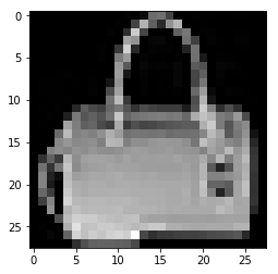
+
When training machine learning models it is important to shuffle the training samples every time you pass through the dataset (i.e. each epoch). Sometimes the order of your samples will have a spurious relationship with the target variable, and shuffling the samples helps remove this. With DataLoader it's as simple as adding `shuffle=True`. You don't need to shuffle the validation and testing data though.
-
-```python
-
+```{.python .input}
batch_size = 32
train_data_loader = mx.gluon.data.DataLoader(train_dataset, batch_size, shuffle=True, num_workers=CPU_COUNT)
valid_data_loader = mx.gluon.data.DataLoader(valid_dataset, batch_size, num_workers=CPU_COUNT)
@@ -147,18 +132,18 @@ Gluon has a number of different Dataset classes for working with your own image
Here you will run through an example for image classification, but a similar process applies for other vision tasks. If you already have your own collection of images to work with you should partition your data into training and test sets, and place all objects of the same class into seperate folders. Similar to:
```
- ./images/train/car/abc.jpg
- ./images/train/car/efg.jpg
- ./images/train/bus/hij.jpg
- ./images/train/bus/klm.jpg
- ./images/test/car/xyz.jpg
- ./images/test/bus/uvw.jpg
+./images/train/car/abc.jpg
+./images/train/car/efg.jpg
+./images/train/bus/hij.jpg
+./images/train/bus/klm.jpg
+./images/test/car/xyz.jpg
+./images/test/bus/uvw.jpg
```
You can download the Caltech 101 dataset if you don't already have images to work with for this example, but please note the download is 126MB.
-```python
+```{.python .input}
data_folder = "data"
dataset_name = "101_ObjectCategories"
archive_file = "{}.tar.gz".format(dataset_name)
@@ -183,18 +168,7 @@ You instantiate the ImageFolderDatasets by providing the path to the data, and t
Optionally, you can pass a `transform` parameter to these `Dataset`'s as you've seen before.
-
-```python
-cd data
-```
-
-
-```python
-!ls
-```
-
-
-```python
+```{.python .input}
training_path='/home/ec2-user/SageMaker/data/101_ObjectCategories'
testing_path='/home/ec2-user/SageMaker/data/101_ObjectCategories_test'
train_dataset = mx.gluon.data.vision.datasets.ImageFolderDataset(training_path)
@@ -206,8 +180,7 @@ Samples from these datasets are tuples of data and label. Images are loaded from
As with the Fashion MNIST dataset the labels will be integer encoded. You can use the `synsets` property of the ImageFolderDatasets to retrieve the original descriptions (e.g. `train_dataset.synsets[i]`).
-```python
-
+```{.python .input}
sample_idx = 539
sample = train_dataset[sample_idx]
data = sample[0]
@@ -222,7 +195,7 @@ imshow(data.asnumpy(), cmap='gray')
```
-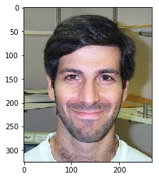<!--notebook-skip-line-->
+<!--notebook-skip-line-->
# Using your own data with custom `Dataset`s
@@ -238,15 +211,12 @@ See [original issue](https://github.com/apache/incubator-mxnet/issues/17269), [p
The current data loading pipeline is the major bottleneck for many training tasks. The flow can be summarized as:
-
-```python
-| Dataset.__getitem__ ->
-| Transform.__call__()/forward() ->
-| Batchify ->
-| (optional communicate through shared_mem) ->
-| split_and_load(ctxs) ->
-| <training on GPUs> ->
-```
+- `Dataset.__getitem__`
+- `Transform.__call__()/forward()`
+- `Batchify`
+- (optional communicate through shared_mem)
+- `split_and_load(ctxs)`
+- training on GPUs
Performance concerns include slow python dataset/transform functions, multithreading issues due to global interpreter lock, Python multiprocessing issues due to speed, and batchify issues due to poor memory management.
@@ -261,16 +231,15 @@ Users can continue to with the traditional gluon.data.Dataloader and the C++ bac
Here you will show a performance increase on a t3.2xl instance for the CIFAR10 dataset with the C++ backend.
-### Using the C++ backend:
-
+## Using the C++ backend:
-```python
+```{.python .input}
cpp_dl = mx.gluon.data.DataLoader(
mx.gluon.data.vision.CIFAR10(train=True, transform=None), batch_size=32, num_workers=2,try_nopython=True)
```
-```python
+```{.python .input}
start = time.time()
for _ in range(3):
print(len(cpp_dl))
@@ -280,16 +249,15 @@ print('Elapsed time for backend dataloader:', time.time() - start)
```
-### Using the Python backend:
+## Using the Python backend:
-
-```python
+```{.python .input}
dl = mx.gluon.data.DataLoader(
mx.gluon.data.vision.CIFAR10(train=True, transform=None), batch_size=32, num_workers=2,try_nopython=False)
```
-```python
+```{.python .input}
start = time.time()
for _ in range(3):
print(len(dl))
@@ -298,10 +266,6 @@ for _ in range(3):
print('Elapsed time for python dataloader:', time.time() - start)
```
-
-### The C++ backend loader was almost 3X faster for this particular use case
-This improvement in performance will not be seen in all cases, but when possible you are encouraged to compare the dataloader throughput for these two options.
-
## Next Steps
-Now that you have some experience with MXNet's datasets and dataloaders, it's time to use them for [Step 6: Training a Neural Network](https://github.com/vidyaravipati/incubator-mxnet/blob/mxnet2.0_crashcourse/docs/python_docs/python/tutorials/getting-started/crash-course/6-train-nn.md).
+Now that you have some experience with MXNet's datasets and dataloaders, it's time to use them for [Step 6: Training a Neural Network](./6-train-nn.ipynb).
diff --git a/docs/python_docs/python/tutorials/getting-started/crash-course/6-train-nn.md b/docs/python_docs/python/tutorials/getting-started/crash-course/6-train-nn.md
index a99fc37..5660de3 100644
--- a/docs/python_docs/python/tutorials/getting-started/crash-course/6-train-nn.md
+++ b/docs/python_docs/python/tutorials/getting-started/crash-course/6-train-nn.md
@@ -29,15 +29,36 @@ and diseased examples of leafs from twelve different plant species. To get this
dataset you have to download and extract it with the following commands.
```{.python .input}
-# Download dataset
-!wget https://md-datasets-cache-zipfiles-prod.s3.eu-west-1.amazonaws.com/hb74ynkjcn-1.zip
+# Import all the necessary libraries to train
+import time
+import os
+import zipfile
+
+import mxnet as mx
+from mxnet import np, npx, gluon, init, autograd
+from mxnet.gluon import nn
+from mxnet.gluon.data.vision import transforms
+
+import matplotlib.pyplot as plt
+import matplotlib.pyplot as plt
+import numpy as np
+
+from prepare_dataset import process_dataset #utility code to rearrange the data
+
+mx.random.seed(42)
```
```{.python .input}
-# Extract the dataset in a folder that create and call plants
-!mkdir plants
-!unzip hb74ynkjcn-1.zip -d plants
-!rm hb74ynkjcn-1.zip
+# Download dataset
+url = 'https://md-datasets-cache-zipfiles-prod.s3.eu-west-1.amazonaws.com/hb74ynkjcn-1.zip'
+zip_file_path = mx.gluon.utils.download(url)
+
+os.makedirs('plants', exist_ok=True)
+
+with zipfile.ZipFile(zip_file_path, 'r') as zf:
+ zf.extractall('plants')
+
+os.remove(zip_file_path)
```
#### Data inspection
@@ -63,43 +84,25 @@ plants
|-- healthy
```
-Each plant species has its own directory, for each of those directories you might
+Each plant species has its own directory, for each of those directories you might
find subdirectories with examples of diseased leaves, healthy
leaves, or both. With this dataset you can formulate different classification
problems; for example, you can create a multi-class classifier that determines
-the species of a plant based on the leaves; you can instead create a binary
-classifier that tells you whether the plant is healthy or diseased. Additionally, you can create
-a multi-class, multi-label classifier that tells you both: what species a
-plant is and whether the plant is diseased or healthy. In this example you will stick to
+the species of a plant based on the leaves; you can instead create a binary
+classifier that tells you whether the plant is healthy or diseased. Additionally, you can create
+a multi-class, multi-label classifier that tells you both: what species a
+plant is and whether the plant is diseased or healthy. In this example you will stick to
the simplest classification question, which is whether a plant is healthy or not.
To do this, you need to manipulate the dataset in two ways. First, you need to
combine all images with labels consisting of healthy and diseased, regardless of the species, and then you
need to split the data into train, validation, and test sets. We prepared a
small utility script that does this to get the dataset ready for you.
-Once you run this utility code on the data, the structure will be
-already organized in folders containing the right images in each of the classes,
+Once you run this utility code on the data, the structure will be
+already organized in folders containing the right images in each of the classes,
you can use the `ImageFolderDataset` class to import the images from the file to MXNet.
```{.python .input}
-# Import all the necessary libraries to train
-import time
-
-import mxnet as mx
-from mxnet import np, npx, gluon, init, autograd
-from mxnet.gluon import nn
-from mxnet.gluon.data.vision import transforms
-
-import matplotlib.pyplot as plt
-import matplotlib.pyplot as plt
-import numpy as np
-
-from prepare_dataset import process_dataset #utility code to rearrange the data
-
-mx.random.seed(42)
-```
-
-```python
# Call the utility function to rearrange the images
process_dataset('plants')
```
@@ -127,7 +130,7 @@ datasets
Now, you need to create three different Dataset objects from the `train`,
`validation`, and `test` folders, and the `ImageFolderDataset` class takes
care of inferring the classes from the directory names. If you don't remember
-how the `ImageFolderDataset` works, take a look at [Step 5](5-datasets.md)
+how the `ImageFolderDataset` works, take a look at [Step 5](5-datasets.md)
of this course for a deeper description.
```{.python .input}
@@ -161,15 +164,16 @@ Usually, you downsize images before passing them to a neural network to reduce t
It is also customary to make slight modifications to the images to improve generalization. That is why you add
transformations to the data in a process called Data Augmentation.
-You can augment data in MXNet using `transforms`. For a complete list of all
-the available transformations in MXNet check out [this link.](https://mxnet.apache.org/versions/1.6/api/python/docs/api/gluon/data/vision/transforms/index.html)
+You can augment data in MXNet using `transforms`. For a complete list of all
+the available transformations in MXNet check out
+[available transforms](../../../api/gluon/data/vision/transforms/index.rst).
It is very common to use more than one transform per image, and it is also
common to process transforms sequentially. To this end, you can use the `transforms.Compose` class.
This class is very useful to create a transformation pipeline for your images.
-You have to compose two different transformation pipelines, one for training
-and the other one for validating and testing. This is because each pipeline
-serves different pursposes. You need to downsize, convert to tensor and normalize
+You have to compose two different transformation pipelines, one for training
+and the other one for validating and testing. This is because each pipeline
+serves different pursposes. You need to downsize, convert to tensor and normalize
images across all the different datsets; however, you typically do not want to randomly flip
or add color jitter to the validation or test images since you could reduce performance.
@@ -204,21 +208,21 @@ With your augmentations ready, you can create the `DataLoaders` to use them. To
do this the `gluon.data.DataLoader` class comes in handy. You have to pass the dataset with
the applied transformations (notice the `.transform_first()` method on the datasets)
to `gluon.data.DataLoader`. Additionally, you need to decide the batch size,
-which is how many images you will be passing to the network,
+which is how many images you will be passing to the network,
and whether you want to shuffle the dataset.
```{.python .input}
# Create data loaders
batch_size = 4
train_loader = gluon.data.DataLoader(train_dataset.transform_first(training_transformer),
- batch_size=batch_size,
- shuffle=True,
+ batch_size=batch_size,
+ shuffle=True,
try_nopython=True)
-validation_loader = gluon.data.DataLoader(val_dataset.transform_first(validation_transformer),
- batch_size=batch_size,
+validation_loader = gluon.data.DataLoader(val_dataset.transform_first(validation_transformer),
+ batch_size=batch_size,
try_nopython=True)
test_loader = gluon.data.DataLoader(test_dataset.transform_first(validation_transformer),
- batch_size=batch_size,
+ batch_size=batch_size,
try_nopython=True)
```
@@ -297,7 +301,7 @@ class LeafNetwork(nn.HybridBlock):
self.dense1 = dense_block(100)
self.dense2 = dense_block(10)
self.dense3 = nn.Dense(2)
-
+
def forward(self, batch):
batch = self.conv1(batch)
batch = self.conv2(batch)
@@ -306,7 +310,7 @@ class LeafNetwork(nn.HybridBlock):
batch = self.dense1(batch)
batch = self.dense2(batch)
batch = self.dense3(batch)
-
+
return batch
```
@@ -318,7 +322,7 @@ hybridize the model.
```{.python .input}
# Create the model based on the blueprint provided and initialize the parameters
-ctx = mx.cpu()
+ctx = mx.cpu()
initializer = mx.initializer.Xavier()
@@ -366,7 +370,7 @@ def test(val_data):
labels = batch[1]
outputs = model(data)
acc.update([labels], [outputs])
-
+
_, accuracy = acc.get()
return accuracy
```
@@ -399,13 +403,13 @@ for epoch in range(epochs):
accuracy.update([label], [outputs])
if log_interval and (idx + 1) % log_interval == 0:
_, acc = accuracy.get()
-
+
print(f"""Epoch[{epoch + 1}] Batch[{idx + 1}] Speed: {batch_size / (time.time() - btic)} samples/sec \
batch loss = {loss.mean().asscalar()} | accuracy = {acc}""")
btic = time.time()
_, acc = accuracy.get()
-
+
acc_val = test(validation_loader)
print(f"[Epoch {epoch + 1}] training: accuracy={acc}")
print(f"[Epoch {epoch + 1}] time cost: {time.time() - tic}")
@@ -435,9 +439,9 @@ parameters in a file. Later, when you want to use the network to make prediction
you can load the parameters back!
```{.python .input}
-# Save parameters in the
+# Save parameters in the
model.save_parameters('leaf_models.params')
```
This is the end of this tutorial, to see how you can speed up the training by
-using GPU hardware continue to the [next tutorial](7-use-gpus.md)
\ No newline at end of file
+using GPU hardware continue to the [next tutorial](./7-use-gpus.ipynb)
diff --git a/docs/python_docs/python/tutorials/getting-started/crash-course/7-use-gpus.md b/docs/python_docs/python/tutorials/getting-started/crash-course/7-use-gpus.md
index c2701c7..babcdd6 100644
--- a/docs/python_docs/python/tutorials/getting-started/crash-course/7-use-gpus.md
+++ b/docs/python_docs/python/tutorials/getting-started/crash-course/7-use-gpus.md
@@ -25,7 +25,7 @@ Before you start the steps, make sure you have at least one Nvidia GPU on your m
You can use the following command to view the number GPUs that are available to MXNet.
-```{.python .input n=2}
+```{.python .input}
from mxnet import np, npx, gluon, autograd
from mxnet.gluon import nn
import time
@@ -38,7 +38,7 @@ npx.num_gpus() #This command provides the number of GPUs MXNet can access
MXNet's ndarray is very similar to NumPy's. One major difference is that MXNet's ndarray has a `context` attribute specifieing which device an array is on. By default, arrays are stored on `npx.cpu()`. To change it to the first GPU, you can use the following code, `npx.gpu()` or `npx.gpu(0)` to indicate the first GPU.
-```{.python .input n=10}
+```{.python .input}
gpu = npx.gpu() if npx.num_gpus() > 0 else npx.cpu()
x = np.ones((3,4), ctx=gpu)
x
@@ -48,7 +48,7 @@ If you're using a CPU, MXNet allocates data on the main memory and tries to use
Assuming there is at least two GPUs. You can create another ndarray and assign it to a different GPU. If you only have one GPU, then you will get an error trying to run this code. In the example code here, you will copy `x` to the second GPU, `npx.gpu(1)`:
-```{.python .input n=11}
+```{.python .input}
gpu_1 = npx.gpu(1) if npx.num_gpus() > 1 else npx.cpu()
x.copyto(gpu_1)
```
@@ -56,13 +56,13 @@ x.copyto(gpu_1)
MXNet requries that users explicitly move data between devices. But several operators such as `print`, and `asnumpy`, will implicitly move data to main memory.
## Choosing GPU Ids
-If you have multiple GPUs on your machine, MXNet can access each of them through 0-indexing with `npx`. As you saw before, the first GPU was accessed using `npx.gpu(0)`, and the second using `npx.gpu(1)`. This extends to however many GPUs your machine has. So if your machine has eight GPUs, the last GPU is accessed using `npx.gpu(7)`. This allows you to select which GPUs to use for operations and training. You might find it particularly useful when you want to leverage multiple GPUs whil [...]
+If you have multiple GPUs on your machine, MXNet can access each of them through 0-indexing with `npx`. As you saw before, the first GPU was accessed using `npx.gpu(0)`, and the second using `npx.gpu(1)`. This extends to however many GPUs your machine has. So if your machine has eight GPUs, the last GPU is accessed using `npx.gpu(7)`. This allows you to select which GPUs to use for operations and training. You might find it particularly useful when you want to leverage multiple GPUs whil [...]
## Run an operation on a GPU
To perform an operation on a particular GPU, you only need to guarantee that the input of an operation is already on that GPU. The output is allocated on the same GPU as well. Almost all operators in the `np` and `npx` module support running on a GPU.
-```{.python .input n=21}
+```{.python .input}
y = np.random.uniform(size=(3,4), ctx=gpu)
x + y
```
@@ -73,7 +73,7 @@ Remember that if the inputs are not on the same GPU, you will get an error.
To run a neural network on a GPU, you only need to copy and move the input data and parameters to the GPU. To demonstrate this you can reuse the previously defined LeafNetwork in [Training Neural Networks](6-train-nn.md). The following code example shows this.
-```{.python .input n=16}
+```{.python .input}
# The convolutional block has a convolution layer, a max pool layer and a batch normalization layer
def conv_block(filters, kernel_size=2, stride=2, batch_norm=True):
conv_block = nn.HybridSequential()
@@ -102,7 +102,7 @@ class LeafNetwork(nn.HybridBlock):
self.dense1 = dense_block(100)
self.dense2 = dense_block(10)
self.dense3 = nn.Dense(2)
-
+
def forward(self, batch):
batch = self.conv1(batch)
batch = self.conv2(batch)
@@ -111,19 +111,19 @@ class LeafNetwork(nn.HybridBlock):
batch = self.dense1(batch)
batch = self.dense2(batch)
batch = self.dense3(batch)
-
+
return batch
```
Load the saved parameters onto GPU 0 directly as shown below; additionally, you could use `net.collect_params().reset_ctx(gpu)` to change the device.
-```{.python .input n=20}
+```{.python .input}
net.load_parameters('leaf_models.params', ctx=gpu)
```
Use the following command to create input data on GPU 0. The forward function will then run on GPU 0.
-```{.python .input n=22}
+```{.python .input}
x = np.random.uniform(size=(1, 3, 128, 128), ctx=gpu)
net(x)
```
@@ -167,7 +167,7 @@ validation_loader = gluon.data.DataLoader(val_dataset.transform_first(validation
test_loader = gluon.data.DataLoader(test_dataset.transform_first(validation_transformer), batch_size=batch_size, try_nopython=True)
```
-### Define a helper function
+### Define a helper function
This is the same test function defined previously in the **Step 6**.
```{.python .input}
@@ -179,7 +179,7 @@ def test(val_data):
labels = batch[1]
outputs = model(data)
acc.update([labels], [outputs])
-
+
_, accuracy = acc.get()
return accuracy
```
@@ -229,19 +229,19 @@ for epoch in range(10):
l.backward()
trainer.step(batch_size)
- # Diff 5: sum losses over all devices. Here, the float
+ # Diff 5: sum losses over all devices. Here, the float
# function will copy data into CPU.
train_loss += sum([float(l.sum()) for l in losses])
accuracy.update(label_list, outputs)
if log_interval and (idx + 1) % log_interval == 0:
_, acc = accuracy.get()
-
+
print(f"""Epoch[{epoch + 1}] Batch[{idx + 1}] Speed: {batch_size / (time.time() - btic)} samples/sec \
batch loss = {train_loss} | accuracy = {acc}""")
btic = time.time()
_, acc = accuracy.get()
-
+
acc_val = test(validation_loader)
print(f"[Epoch {epoch + 1}] training: accuracy={acc}")
print(f"[Epoch {epoch + 1}] time cost: {time.time() - tic}")
@@ -250,4 +250,7 @@ for epoch in range(10):
## Next steps
-Now that you have completed training and predicting with a neural network on GPUs, you can dive deep into other gluon packages: [GluonCV](https://cv.gluon.ai/tutorials/index.html) and [GluonNLP](https://nlp.gluon.ai) if you want to understand those better. Otherwise, this is the conclusion of the crash course.
+Now that you have completed training and predicting with a neural network on GPUs, you reached the conclusion of the crash course. Congratulations.
+If you are keen on studying more, checkout [D2L.ai](https://d2l.ai),
+[GluonCV](https://cv.gluon.ai/tutorials/index.html), [GluonNLP](https://nlp.gluon.ai),
+[GluonTS](https://ts.gluon.ai/), [AutoGluon](https://auto.gluon.ai).
diff --git a/docs/python_docs/python/tutorials/getting-started/gluon_from_experiment_to_deployment.md b/docs/python_docs/python/tutorials/getting-started/gluon_from_experiment_to_deployment.md
index 7f34708..8d583eb 100644
--- a/docs/python_docs/python/tutorials/getting-started/gluon_from_experiment_to_deployment.md
+++ b/docs/python_docs/python/tutorials/getting-started/gluon_from_experiment_to_deployment.md
@@ -20,7 +20,6 @@
## Overview
MXNet Gluon API comes with a lot of great features, and it can provide you everything you need: from experimentation to deploying the model. In this tutorial, we will walk you through a common use case on how to build a model using gluon, train it on your data, and deploy it for inference.
-This tutorial covers training and inference in Python, please continue to [C++ inference part](/api/cpp/docs/tutorials/cpp_inference) after you finish.
Let's say you need to build a service that provides flower species recognition. A common problem is that you don't have enough data to train a good model. In such cases, a technique called Transfer Learning can be used to make a more robust model.
In Transfer Learning we make use of a pre-trained model that solves a related task, and was trained on a very large standard dataset, such as ImageNet. ImageNet is from a different domain, but we can utilize the knowledge in this pre-trained model to perform the new task at hand.
@@ -77,7 +76,7 @@ from mxnet.gluon.data.vision import transforms
from mxnet.gluon.model_zoo.vision import resnet50_v2
```
-Next, we define the hyper-parameters that we will use for fine-tuning. We will use the [MXNet learning rate scheduler](/api/python/docs/tutorials/packages/gluon/training/learning_rates/learning_rate_schedules.html) to adjust learning rates during training.
+Next, we define the hyper-parameters that we will use for fine-tuning. We will use the [MXNet learning rate scheduler](../packages/gluon/training/learning_rates/learning_rate_schedules.ipynb) to adjust learning rates during training.
Here we set the `epochs` to 1 for quick demonstration, please change to 40 for actual training.
```{.python .input}
@@ -99,14 +98,14 @@ ctx = [mx.gpu(i) for i in range(num_gpus)] if num_gpus > 0 else [mx.cpu()]
batch_size = per_device_batch_size * max(num_gpus, 1)
```
-Now we will apply data augmentations on training images. This makes minor alterations on the training images, and our model will consider them as distinct images. This can be very useful for fine-tuning on a relatively small dataset, and it will help improve the model. We can use the Gluon [DataSet API](/api/python/docs/api/gluon/data/index.html#mxnet.gluon.data.Dataset), [DataLoader API](/api/python/docs/api/gluon/data/index.html#mxnet.gluon.data.DataLoader), and [Transform API](/api/py [...]
+Now we will apply data augmentations on training images. This makes minor alterations on the training images, and our model will consider them as distinct images. This can be very useful for fine-tuning on a relatively small dataset, and it will help improve the model. We can use the Gluon [DataSet API](../../api/gluon/data/index.rst#mxnet.gluon.data.Dataset), [DataLoader API](../../api/gluon/data/index.rst#mxnet.gluon.data.DataLoader), and [Transform API](../../api/gluon/data/index.rst# [...]
1. Randomly crop the image and resize it to 224x224
2. Randomly flip the image horizontally
3. Randomly jitter color and add noise
4. Transpose the data from `[height, width, num_channels]` to `[num_channels, height, width]`, and map values from [0, 255] to [0, 1]
5. Normalize with the mean and standard deviation from the ImageNet dataset.
-For validation and inference, we only need to apply step 1, 4, and 5. We also need to save the mean and standard deviation values for [inference using C++](/api/cpp/docs/tutorials/cpp_inference).
+For validation and inference, we only need to apply step 1, 4, and 5. We also need to save the mean and standard deviation values for inference using other language bindings.
```{.python .input}
jitter_param = 0.4
@@ -161,7 +160,7 @@ test_data = gluon.data.DataLoader(
We will use pre-trained ResNet50_v2 model which was pre-trained on the [ImageNet Dataset](http://www.image-net.org/) with 1000 classes. To match the classes in the Flower dataset, we must redefine the last softmax (output) layer to be 102, then initialize the parameters.
-Before we go to training, one unique Gluon feature you should be aware of is hybridization. It allows you to convert your imperative code to a static symbolic graph, which is much more efficient to execute. There are two main benefits of hybridizing your model: better performance and easier serialization for deployment. The best part is that it's as simple as just calling `net.hybridize()`. To know more about Gluon hybridization, please follow the [hybridization tutorial](/api/python/doc [...]
+Before we go to training, one unique Gluon feature you should be aware of is hybridization. It allows you to convert your imperative code to a static symbolic graph, which is much more efficient to execute. There are two main benefits of hybridizing your model: better performance and easier serialization for deployment. The best part is that it's as simple as just calling `net.hybridize()`. To know more about Gluon hybridization, please follow the [hybridization tutorial](../packages/glu [...]
@@ -263,17 +262,13 @@ finetune_net.export("flower-recognition", epoch=epochs)
## What's next
-You can continue to the [next tutorial](/api/cpp/docs/tutorials/cpp_inference) on how to load the model we just trained and run inference using MXNet C++ API.
-
-You can also find more ways to run inference and deploy your models here:
-1. [Java Inference examples](https://github.com/apache/incubator-mxnet/tree/master/scala-package/examples/src/main/java/org/apache/mxnetexamples/javaapi/infer)
-2. [Scala Inference examples](/api/scala/docs/tutorials/infer)
-4. [MXNet Model Server Examples](https://github.com/awslabs/mxnet-model-server/tree/master/examples)
+You can find more ways to run inference and deploy your models here:
+1. [MXNet Model Server Examples](https://github.com/awslabs/mxnet-model-server/tree/master/examples)
## References
1. [Transfer Learning for Oxford102 Flower Dataset](https://github.com/Arsey/keras-transfer-learning-for-oxford102)
2. [Gluon book on fine-tuning](https://www.d2l.ai/chapter_computer-vision/fine-tuning.html)
-3. [Gluon CV transfer learning tutorial](https://gluon-cv.mxnet.io/build/examples_classification/transfer_learning_minc.html)
+3. [Gluon CV transfer learning tutorial](https://cv.gluon.ai/build/examples_classification/transfer_learning_minc.html)
4. [Gluon crash course](https://gluon-crash-course.mxnet.io/)
5. [Gluon CPP inference example](https://github.com/apache/incubator-mxnet/blob/master/cpp-package/example/inference/)
diff --git a/docs/python_docs/python/tutorials/getting-started/logistic_regression_explained.md b/docs/python_docs/python/tutorials/getting-started/logistic_regression_explained.md
index e36e048..94aff3d 100644
--- a/docs/python_docs/python/tutorials/getting-started/logistic_regression_explained.md
+++ b/docs/python_docs/python/tutorials/getting-started/logistic_regression_explained.md
@@ -55,7 +55,7 @@ batch_size = 10
## Working with data
-To work with data, Apache MXNet provides [Dataset](https://mxnet.apache.org/api/python/gluon/data.html#mxnet.gluon.data.Dataset) and [DataLoader](https://mxnet.apache.org/api/python/gluon/data.html#mxnet.gluon.data.DataLoader) classes. The former is used to provide an indexed access to the data, the latter is used to shuffle and batchify the data. To learn more about working with data in Gluon, please refer to [Gluon Datasets and Dataloaders](/api/python/docs/api/gluon/data/index.html).
+To work with data, Apache MXNet provides [Dataset](../../api/gluon/data/index.rst#mxnet.gluon.data.Dataset) and [DataLoader](../../api/gluon/data/index.rst#mxnet.gluon.data.DataLoader) classes. The former is used to provide an indexed access to the data, the latter is used to shuffle and batchify the data. To learn more about working with data in Gluon, please refer to [Gluon Datasets and Dataloaders](../../api/gluon/data/index.rst).
Below we define training and validation datasets, which we are going to use in the tutorial.
@@ -72,9 +72,9 @@ val_dataloader = DataLoader(val_dataset, batch_size=batch_size, shuffle=True)
## Defining and training the model
-The only requirement for the logistic regression is that the last layer of the network must be a single neuron. Apache MXNet allows us to do so by using [Dense](https://mxnet.apache.org/api/python/gluon/nn.html#mxnet.gluon.nn.Dense) layer and specifying the number of units to 1. The rest of the network can be arbitrarily complex.
+The only requirement for the logistic regression is that the last layer of the network must be a single neuron. Apache MXNet allows us to do so by using [Dense](../../api/gluon/nn/index.rst#mxnet.gluon.nn.Dense) layer and specifying the number of units to 1. The rest of the network can be arbitrarily complex.
-Below, we define a model which has an input layer of 10 neurons, a couple of inner layers of 10 neurons each, and output layer of 1 neuron. We stack the layers using [HybridSequential](https://mxnet.apache.org/api/python/gluon/gluon.html#mxnet.gluon.nn.HybridSequential) block and initialize parameters of the network using [Xavier](https://mxnet.apache.org/api/python/optimization/optimization.html#mxnet.initializer.Xavier) initialization.
+Below, we define a model which has an input layer of 10 neurons, a couple of inner layers of 10 neurons each, and output layer of 1 neuron. We stack the layers using [HybridSequential](../../api/gluon/nn/index.rst#mxnet.gluon.nn.HybridSequential) block and initialize parameters of the network using [Xavier](../../api/initializer/index.rst#mxnet.initializer.Xavier) initialization.
```{.python .input}
@@ -90,11 +90,11 @@ net.initialize(mx.init.Xavier())
After defining the model, we need to define a few more things: our loss, our trainer and our metric.
-Loss function is used to calculate how the output of the network differs from the ground truth. Because classes of the logistic regression are either 0 or 1, we are using [SigmoidBinaryCrossEntropyLoss](https://mxnet.apache.org/api/python/gluon/loss.html#mxnet.gluon.loss.SigmoidBinaryCrossEntropyLoss). Notice that we do not specify `from_sigmoid` attribute in the code, which means that the output of the neuron doesn't need to go through sigmoid, but at inference we'd have to pass it thr [...]
+Loss function is used to calculate how the output of the network differs from the ground truth. Because classes of the logistic regression are either 0 or 1, we are using [SigmoidBinaryCrossEntropyLoss](../../api/gluon/loss/index.rst#mxnet.gluon.loss.SigmoidBinaryCrossEntropyLoss). Notice that we do not specify `from_sigmoid` attribute in the code, which means that the output of the neuron doesn't need to go through sigmoid, but at inference we'd have to pass it through sigmoid. You can [...]
-Trainer object allows to specify the method of training to be used. For our tutorial we use [Stochastic Gradient Descent (SGD)](https://mxnet.apache.org/api/python/optimization/optimization.html#mxnet.optimizer.SGD). For more information on SGD refer to [the following tutorial](https://gluon.mxnet.io/chapter06_optimization/gd-sgd-scratch.html). We also need to parametrize it with learning rate value, which defines the weight updates, and weight decay, which is used for regularization.
+Trainer object allows to specify the method of training to be used. For our tutorial we use [Stochastic Gradient Descent (SGD)](../../api/optimizer/index.rst#mxnet.optimizer.SGD). For more information on SGD refer to [the following tutorial](https://gluon.mxnet.io/chapter06_optimization/gd-sgd-scratch.html). We also need to parametrize it with learning rate value, which defines the weight updates, and weight decay, which is used for regularization.
-Metric helps us to estimate how good our model is in terms of a problem we are trying to solve. Where loss function has more importance for the training process, a metric is usually the thing we are trying to improve and reach maximum value. We also can use more than one metric, to measure various aspects of our model. In our example, we are using [Accuracy](https://mxnet.apache.org/api/python/metric/metric.html?highlight=metric.acc#mxnet.metric.Accuracy) and [F1 score](http://mxnet.apac [...]
+Metric helps us to estimate how good our model is in terms of a problem we are trying to solve. Where loss function has more importance for the training process, a metric is usually the thing we are trying to improve and reach maximum value. We also can use more than one metric, to measure various aspects of our model. In our example, we are using [Accuracy](../../api/gluon/metric/index.rst#mxnet.gluon.metric.Accuracy) and [F1 score](../../api/gluon/metric/index.rst#mxnet.gluon.metric.F1 [...]
Below we define these objects.
@@ -136,17 +136,17 @@ def train_model():
## Validating the model
-Our validation function is very similar to the training one. The main difference is that we want to calculate accuracy of the model. We use [Accuracy metric](https://mxnet.apache.org/api/python/metric/metric.html?highlight=metric.acc#mxnet.metric.Accuracy) to do so.
+Our validation function is very similar to the training one. The main difference is that we want to calculate accuracy of the model. We use [Accuracy metric](../../api/gluon/metric/index.rst#mxnet.gluon.metric.Accuracy) to do so.
`Accuracy` metric requires 2 arguments: 1) a vector of ground-truth classes and 2) A vector or matrix of predictions. When predictions are of the same shape as the vector of ground-truth classes, `Accuracy` class assumes that prediction vector contains predicted classes. So, it converts the vector to `Int32` and compare each item of ground-truth classes to prediction vector.
-Because of the behaviour above, you will get an unexpected result if you just apply [Sigmoid](https://mxnet.apache.org/api/python/ndarray/ndarray.html#mxnet.ndarray.sigmoid) function to the network result and pass it to `Accuracy` metric. As mentioned before, we need to apply `Sigmoid` function to the output of the neuron to get a probability of belonging to the class 1. But `Sigmoid` function produces output in range [0; 1], and all numbers in that range are going to be casted to 0, eve [...]
+Because of the behaviour above, you will get an unexpected result if you just apply [Sigmoid](../../api/legacy/ndarray/ndarray.rst#mxnet.ndarray.sigmoid) function to the network result and pass it to `Accuracy` metric. As mentioned before, we need to apply `Sigmoid` function to the output of the neuron to get a probability of belonging to the class 1. But `Sigmoid` function produces output in range [0; 1], and all numbers in that range are going to be casted to 0, even if it is as high a [...]
1. Calculates sigmoid using `Sigmoid` function
2. Subtracts a threshold from the original sigmoid output. Usually, the threshold is equal to 0.5, but it can be higher, if you want to increase certainty of an item to belong to class 1.
-3. Uses [mx.nd.ceil](https://mxnet.apache.org/api/python/ndarray/ndarray.html#mxnet.ndarray.ceil) function, which converts all negative values to 0 and all positive values to 1
+3. Uses [mx.nd.ceil](../../api/legacy/ndarray/ndarray.rst#mxnet.ndarray.ceil) function, which converts all negative values to 0 and all positive values to 1
After these transformations we can pass the result to `Accuracy.update()` method and expect it to behave in a proper way.
@@ -244,7 +244,7 @@ For `SigmoidBinaryCrossEntropyLoss` to work it is required that classes were enc
## Tip 3: Use SigmoidBinaryCrossEntropyLoss
-NDArray API has an options to calculate logistic regression loss: [SigmoidBinaryCrossEntropyLoss](https://mxnet.apache.org/api/python/gluon/loss.html#mxnet.gluon.loss.SigmoidBinaryCrossEntropyLoss).
+Gluon API has an options to calculate logistic regression loss: [SigmoidBinaryCrossEntropyLoss](../../api/gluon/loss/index.rst#mxnet.gluon.loss.SigmoidBinaryCrossEntropyLoss).
## Conclusion
diff --git a/docs/python_docs/python/tutorials/getting-started/to-mxnet/pytorch.md b/docs/python_docs/python/tutorials/getting-started/to-mxnet/pytorch.md
index aada149..a374d93 100644
--- a/docs/python_docs/python/tutorials/getting-started/to-mxnet/pytorch.md
+++ b/docs/python_docs/python/tutorials/getting-started/to-mxnet/pytorch.md
@@ -19,7 +19,7 @@
[PyTorch](https://pytorch.org/) is a popular deep learning framework due to its easy-to-understand API and its completely imperative approach. Apache MXNet includes the Gluon API which gives you the simplicity and flexibility of PyTorch and allows you to hybridize your network to leverage performance optimizations of the symbolic graph. As of April 2019, [NVidia performance benchmarks](https://developer.nvidia.com/deep-learning-performance-training-inference) show that Apache MXNet outpe [...]
-In the next 10 minutes, we'll do a quick comparison between the two frameworks and show how small the learning curve can be when switching from PyTorch to Apache MXNet.
+In the next 10 minutes, we'll do a quick comparison between the two frameworks and show how small the learning curve can be when switching from PyTorch to Apache MXNet.
## Installation
@@ -106,7 +106,7 @@ mx_train_data = gluon.data.DataLoader(
Both frameworks allows you to download MNIST data set from their sources and specify that only training part of the data set is required.
-The main difference between the code snippets is that MXNet uses [transform_first](/api/python/docs/api/gluon/data/index.html#mxnet.gluon.data.Dataset.transform_first) method to indicate that the data transformation is done on the first element of the data batch, the MNIST picture, rather than the second element, the label.
+The main difference between the code snippets is that MXNet uses [transform_first](../../../api/gluon/data/index.rst#mxnet.gluon.data.Dataset.transform_first) method to indicate that the data transformation is done on the first element of the data batch, the MNIST picture, rather than the second element, the label.
### 2. Creating the model
@@ -143,7 +143,7 @@ We used the Sequential container to stack layers one after the other in order to
* After the model structure is defined, Apache MXNet requires you to explicitly call the model initialization function.
-With a Sequential block, layers are executed one after the other. To have a different execution model, with PyTorch you can inherit from `nn.Module` and then customize how the `.forward()` function is executed. Similarly, in Apache MXNet you can inherit from [nn.Block](/api/python/docs/api/gluon/nn/index.html#mxnet.gluon.nn.Block) to achieve similar results.
+With a Sequential block, layers are executed one after the other. To have a different execution model, with PyTorch you can inherit from `nn.Module` and then customize how the `.forward()` function is executed. Similarly, in Apache MXNet you can inherit from [gluon.Block](../../../api/gluon/block.rst#mxnet.gluon.Block) to achieve similar results.
### 3. Loss function and optimization algorithm
@@ -164,7 +164,7 @@ mx_trainer = gluon.Trainer(mx_net.collect_params(),
'sgd', {'learning_rate': 0.1})
```
-The code difference between frameworks is small. The main difference is that in Apache MXNet we use [Trainer](/api/python/docs/api/gluon/trainer.html) class, which accepts optimization algorithm as an argument. We also use [.collect_params()](/api/python/docs/api/gluon/block.html#mxnet.gluon.Block.collect_params) method to get parameters of the network.
+The code difference between frameworks is small. The main difference is that in Apache MXNet we use [Trainer](../../../api/gluon/trainer.rst) class, which accepts optimization algorithm as an argument. We also use [.collect_params()](../../../api/gluon/block.rst#mxnet.gluon.Block.collect_params) method to get parameters of the network.
### 4. Training
@@ -212,13 +212,13 @@ Some of the differences in Apache MXNet when compared to PyTorch are as follows:
* In Apache MXNet, you don't need to flatten the 4-D input into 2-D when feeding the data into forward pass.
-* In Apache MXNet, you need to perform the calculation within the [autograd.record()](/api/python/docs/api/autograd/index.html?autograd%20record#mxnet.autograd.record) scope so that it can be automatically differentiated in the backward pass.
+* In Apache MXNet, you need to perform the calculation within the [autograd.record()](../../../api/autograd/index.rst#mxnet.autograd.record) scope so that it can be automatically differentiated in the backward pass.
* It is not necessary to clear the gradient every time as with PyTorch's `trainer.zero_grad()` because by default the new gradient is written in, not accumulated.
-* You need to specify the update step size (usually batch size) when performing [step()](/api/python/docs/api/gluon/trainer.html?#mxnet.gluon.Trainer.step) on the trainer.
+* You need to specify the update step size (usually batch size) when performing [step()](../../../api/gluon/trainer.rst#mxnet.gluon.Trainer.step) on the trainer.
-* You need to call [.asscalar()](/api/python/docs/api/ndarray/ndarray.html?#mxnet.ndarray.NDArray.asscalar) to turn a multidimensional array into a scalar.
+* You need to call [.asscalar()](../../../api/legacy/ndarray/ndarray.rst#mxnet.ndarray.NDArray.asscalar) to turn a multidimensional array into a scalar.
* In this sample, Apache MXNet is twice as fast as PyTorch. Though you need to be cautious with such toy comparisons.
@@ -230,9 +230,9 @@ As we saw above, Apache MXNet Gluon API and PyTorch have many similarities. The
While Apache MXNet Gluon API is very similar to PyTorch, there are some extra functionality that can make your code even faster.
-* Check out [Hybridize tutorial](/api/python/docs/tutorials/packages/gluon/blocks/hybridize.html) to learn how to write imperative code which can be converted to symbolic one.
+* Check out [Hybridize tutorial](../../packages/gluon/blocks/hybridize.ipynb) to learn how to write imperative code which can be converted to symbolic one.
-* Also, check out how to extend Apache MXNet with your own [custom layers](/api/python/docs/tutorials/packages/gluon/blocks/custom-layer.html?custom_layers).
+* Also, check out how to extend Apache MXNet with your own [custom layers](../../packages/gluon/blocks/custom-layer.ipynb).
## Appendix
diff --git a/docs/python_docs/python/tutorials/packages/autograd/index.md b/docs/python_docs/python/tutorials/packages/autograd/index.md
index 155fb4f..91d7cbd 100644
--- a/docs/python_docs/python/tutorials/packages/autograd/index.md
+++ b/docs/python_docs/python/tutorials/packages/autograd/index.md
@@ -23,21 +23,21 @@
Gradients are fundamental to the process of training neural networks, and tell us how to change the parameters of the network to improve its performance.
-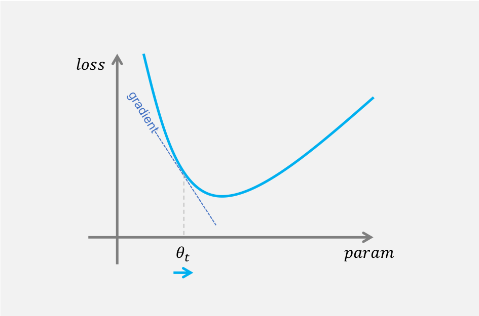
+
### Long Answer:
Under the hood, neural networks are composed of operators (e.g. sums, products, convolutions, etc) some of which use parameters (e.g. the weights in convolution kernels) for their computation, and it's our job to find the optimal values for these parameters. Gradients lead us to the solution!
-Gradients tell us how much a given variable increases or decreases when we change a variable it depends on. What we're interested in is the effect of changing a each parameter on the performance of the network. We usually define performance using a loss metric that we try to minimize, i.e. a metric that tells us how bad the predictions of a network are given ground truth. As an example, for regression we might try to minimize the [L2 loss](/api/python/docs/api/gluon/loss/index.html#mxnet [...]
+Gradients tell us how much a given variable increases or decreases when we change a variable it depends on. What we're interested in is the effect of changing a each parameter on the performance of the network. We usually define performance using a loss metric that we try to minimize, i.e. a metric that tells us how bad the predictions of a network are given ground truth. As an example, for regression we might try to minimize the [L2 loss](../../../api/gluon/loss/index.rst#mxnet.gluon.lo [...]
-Assuming we've calculated the gradient of each parameter with respect to the loss (details in next section), we can then use an optimizer such as [stochastic gradient descent](https://en.wikipedia.org/wiki/Stochastic_gradient_descent) to shift the parameters slightly in the *opposite direction* of the gradient. See [Optimizers](/api/python/docs/api/optimizer/index.html) for more information on these methods. We repeat the process of calculating gradients and updating parameters over and [...]
+Assuming we've calculated the gradient of each parameter with respect to the loss (details in next section), we can then use an optimizer such as [stochastic gradient descent](https://en.wikipedia.org/wiki/Stochastic_gradient_descent) to shift the parameters slightly in the *opposite direction* of the gradient. See [Optimizers](../../../api/optimizer/index.rst) for more information on these methods. We repeat the process of calculating gradients and updating parameters over and over agai [...]
## How do we calculate gradients?
### Short Answer:
-We differentiate. [MXNet Gluon](/api/python/docs/tutorials/packages/gluon/index.html) uses Reverse Mode Automatic Differentiation (`autograd`) to backprogate gradients from the loss metric to the network parameters.
+We differentiate. [MXNet Gluon](../gluon/index.ipynb) uses Reverse Mode Automatic Differentiation (`autograd`) to backprogate gradients from the loss metric to the network parameters.
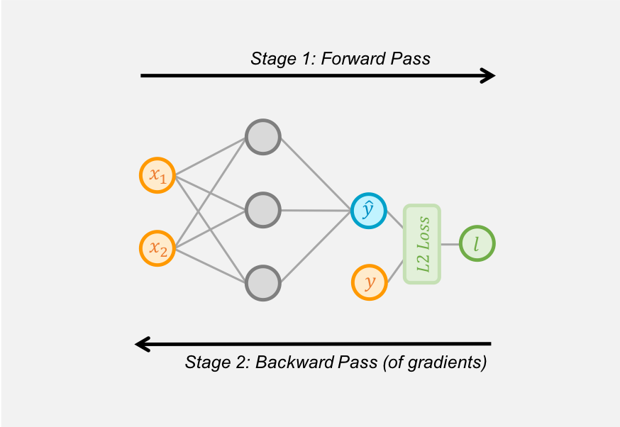
@@ -159,7 +159,7 @@ print('is_training:', is_training, output)
We called `dropout` while `autograd` was recording this time, so our network was in training mode and we see dropout of the input this time. Since the probability of dropout was 50%, the output is automatically scaled by 1/0.5=2 to preserve the average activation.
-We can force some operators to behave as they would during training, even in inference mode. One example is setting `mode='always'` on the [Dropout](/api/python/ndarray/ndarray.html#mxnet.ndarray.Dropout) operator, but this usage is uncommon.
+We can force some operators to behave as they would during training, even in inference mode. One example is setting `mode='always'` on the [Dropout](../../../api/legacy/ndarray/ndarray.rst#mxnet.ndarray.Dropout) operator, but this usage is uncommon.
## Advanced: Skipping the calculation of parameter gradients
@@ -196,7 +196,7 @@ print(x.grad)
## Advanced: Using Python control flow
-As mentioned before, one of the main advantages of `autograd` is the ability to automatically calculate gradients of dynamic graphs (i.e. graphs where the operators could be different on every forward pass). One example of this would be applying a tree structured recurrent network to parse a sentence using its parse tree. And we can use Python control flow operators to create a dynamic flow that depends on the data, rather than using [MXNet's control flow operators](/api/python/docs/tuto [...]
+As mentioned before, one of the main advantages of `autograd` is the ability to automatically calculate gradients of dynamic graphs (i.e. graphs where the operators could be different on every forward pass). One example of this would be applying a tree structured recurrent network to parse a sentence using its parse tree. And we can use Python control flow operators to create a dynamic flow that depends on the data, rather than using MXNet's control flow operators.
We'll write a function as a toy example of a dynamic network. We'll add an `if` condition and a loop with a variable number of iterations, both of which will depend on the input data. Although these can now be used in static graphs (with conditional operators) it's still much more natural to use native control flow.
diff --git a/docs/python_docs/python/tutorials/packages/gluon/blocks/activations/activations.md b/docs/python_docs/python/tutorials/packages/gluon/blocks/activations/activations.md
index 13a4830..35642a1 100644
--- a/docs/python_docs/python/tutorials/packages/gluon/blocks/activations/activations.md
+++ b/docs/python_docs/python/tutorials/packages/gluon/blocks/activations/activations.md
@@ -17,7 +17,7 @@
# Activation Blocks
-Deep neural networks are a way to express a nonlinear function with lots of parameters from input data to outputs. The nonlinearities that allow neural networks to capture complex patterns in data are referred to as activation functions. Over the course of the development of neural networks, several nonlinear activation functions have been introduced to make gradient-based deep learning tractable.
+Deep neural networks are a way to express a nonlinear function with lots of parameters from input data to outputs. The nonlinearities that allow neural networks to capture complex patterns in data are referred to as activation functions. Over the course of the development of neural networks, several nonlinear activation functions have been introduced to make gradient-based deep learning tractable.
If you are looking to answer the question, 'which activation function should I use for my neural network model?', you should probably go with *ReLU*. Unless you're trying to implement something like a gating mechanism, like in LSTMs or GRU cells, then you should opt for sigmoid and/or tanh in those cells. However, if you have a working model architecture and you're trying to improve its performance by swapping out activation functions or treating the activation function as a hyperparamet [...]
@@ -38,20 +38,20 @@ def visualize_activation(activation_fn):
with mx.autograd.record():
y = activation_fn(x)
y.backward()
-
+
plt.figure()
plt.plot(data, y.asnumpy())
plt.plot(data, x.grad.asnumpy())
activation = activation_fn.name[:-1]
plt.legend(["{} activation".format(activation), "{} gradient".format(activation)])
-
+
```
## Sigmoids
### Sigmoid
-The sigmoid activation function, also known as the logistic function or logit function, is perhaps the most widely known activation owing to its [long history](https://web.stanford.edu/class/psych209a/ReadingsByDate/02_06/PDPVolIChapter8.pdf) in neural network training and appearance in logistic regression and kernel methods for classification.
+The sigmoid activation function, also known as the logistic function or logit function, is perhaps the most widely known activation owing to its [long history](https://web.stanford.edu/class/psych209a/ReadingsByDate/02_06/PDPVolIChapter8.pdf) in neural network training and appearance in logistic regression and kernel methods for classification.
The sigmoid activation is a non-linear function that transforms any real valued input to a value between 0 and 1, giving it a natural probabilistic interpretation. The sigmoid takes the form of the function below.
@@ -67,17 +67,17 @@ visualize_activation(mx.gluon.nn.Activation('sigmoid'))
```
-
+
-The sigmoid activation has since fallen out of use as the preferred activation function in designing neural networks due to some of its properties, shown in the plot above, like not being zero-centered and inducing vanishing gradients, that leads to poor performance during neural network training. Vanishing gradients here refers to the tendency of the gradient of the sigmoid function to be nearly zero for most input values.
+The sigmoid activation has since fallen out of use as the preferred activation function in designing neural networks due to some of its properties, shown in the plot above, like not being zero-centered and inducing vanishing gradients, that leads to poor performance during neural network training. Vanishing gradients here refers to the tendency of the gradient of the sigmoid function to be nearly zero for most input values.
### tanh
The tanh, or hyperbolic tangent, activation function is also an s shaped curve albeit one whose output values range from -1 to 1. It is defined by the mathematical equation:
-$$ tanh(x) = \dfrac{e^x - e^{-x}}{e^x + e^{-x}}$$
+$$ tanh(x) = \dfrac{e^x - e^{-x}}{e^x + e^{-x}}$$
-tanh addresses the issues of not being zero centered associated with the sigmoid activation function but still retains the vanishing gradient problems due to the gradient being asymptotically zero for values outside a narrow range of inputs.
+tanh addresses the issues of not being zero centered associated with the sigmoid activation function but still retains the vanishing gradient problems due to the gradient being asymptotically zero for values outside a narrow range of inputs.
In fact, the tanh can be rewritten as,
@@ -95,7 +95,7 @@ visualize_activation(mx.gluon.nn.Activation('tanh'))
```
-
+
The use of tanh as activation functions in place of the logistic function was popularized by the success of the [LeNet architecture](http://yann.lecun.com/exdb/publis/pdf/lecun-01a.pdf) and the [methods paper](http://yann.lecun.com/exdb/publis/pdf/lecun-98b.pdf) by LeCun et al.
@@ -112,7 +112,7 @@ visualize_activation(mx.gluon.nn.Activation('softsign'))
```
-
+
The softsign function is not a commonly used activation with most neural networks and still suffers from the vanishing gradient problem as seen in the graph above.
@@ -134,7 +134,7 @@ visualize_activation(mx.gluon.nn.Activation('relu'))
```
-
+
As shown above, the ReLU activation mitigates the vanishing gradient problem associated with the sigmoid family of activations, by having a larger (infinite) range of values where its gradient is non-zero. However, one drawback of ReLU as an activation function is a phenomenon referred to as the 'Dying ReLU', where gradient-based parameter updates can happen in such a way that the gradient flowing through a ReLU unit is always zero and the connection is never activated. This can largely [...]
@@ -153,7 +153,7 @@ visualize_activation(mx.gluon.nn.Activation('softrelu'))
```
-
+
### Leaky ReLU
@@ -163,7 +163,7 @@ Leaky ReLUs are a variant of ReLU that multiply the input by a small positive pa
$$ LeakyReLU(\alpha, x) = \begin{cases}
x,& \text{if } x\geq 0\\
\alpha x, & \text{otherwise}
-\end{cases}$$
+\end{cases}$$
where $\alpha > 0$ is small positive number. In MXNet, by default the $\alpha$ parameter is set to 0.01.
@@ -175,7 +175,7 @@ visualize_activation(mx.gluon.nn.LeakyReLU(0.05))
```
-
+
As shown in the graph, the LeakyReLU's gradient is non-zero everywhere, in an attempt to address the ReLU's gradient being zero for all negative values.
@@ -191,14 +191,14 @@ visualize_activation(prelu)
```
-
+
The activation function and activation gradient of PReLU have the same shape as LeakyRELU.
### ELU
-The ELU or exponential linear unit introduced by [Clevert et al](https://arxiv.org/abs/1511.07289) also addresses the vanishing gradient problem like ReLU and its variants but unlike the ReLU family, ELU allows negative values which may allow them to push mean unit activations closer to zero like batch normalization.
+The ELU or exponential linear unit introduced by [Clevert et al](https://arxiv.org/abs/1511.07289) also addresses the vanishing gradient problem like ReLU and its variants but unlike the ReLU family, ELU allows negative values which may allow them to push mean unit activations closer to zero like batch normalization.
The ELU function has the form
@@ -213,7 +213,7 @@ visualize_activation(mx.gluon.nn.ELU())
```
-
+
### SELU
@@ -234,7 +234,7 @@ visualize_activation(mx.gluon.nn.SELU())
```
-
+
### SiLU
@@ -252,7 +252,7 @@ visualize_activation(mx.gluon.nn.SiLU())
```
-
+
### GELU
The GELU is a smooth approximation to the ReLU and was introduced in [Hendrycks et al](https://arxiv.org/abs/1606.08415). It is a common activation function in architectures such as Transformers, BERT, and GPT.
@@ -270,7 +270,7 @@ Note $\Phi(x) = \frac{1}{\sqrt{2 \pi}} \exp\left\{-\frac{x^2}{2}\right\}$ is the
visualize_activation(mx.gluon.nn.GELU())
```
-
+
## Summary
@@ -286,7 +286,7 @@ visualize_activation(mx.gluon.nn.GELU())
## Next Steps
Activations are just one component of neural network architectures. Here are a few MXNet resources to learn more about activation functions and how they they combine with other components of neural nets.
-* Learn how to create a Neural Network with these activation layers and other neural network layers in the [gluon crash course](/api/python/docs/tutorials/getting-started/crash-course/index.html).
-* Check out the guide to MXNet [gluon layers and blocks](/api/python/docs/tutorials/packages/gluon/blocks/nn.html) to learn about the other neural network layers in implemented in MXNet and how to create custom neural networks with these layers.
-* Also check out the [guide to normalization layers](/api/python/docs/tutorials/packages/gluon/training/normalization/index.html) to learn about neural network layers that normalize their inputs.
-* Finally take a look at the [Custom Layer guide](/api/python/docs/tutorials/extend/custom_layer.html) to learn how to implement your own custom activation layer.
+* Learn how to create a Neural Network with these activation layers and other neural network layers in the [Gluon crash course](../../../../getting-started/crash-course/index.ipynb).
+* Check out the guide to MXNet [gluon layers and blocks](../nn.ipynb) to learn about the other neural network layers in implemented in MXNet and how to create custom neural networks with these layers.
+* Also check out the [guide to normalization layers](../../training/normalization/index.ipynb) to learn about neural network layers that normalize their inputs.
+* Finally take a look at the [Custom Layer guide](../custom-layer.ipynb) to learn how to implement your own custom activation layer.
diff --git a/docs/python_docs/python/tutorials/packages/gluon/blocks/custom-layer.md b/docs/python_docs/python/tutorials/packages/gluon/blocks/custom-layer.md
index ff62a55..2e37826 100644
--- a/docs/python_docs/python/tutorials/packages/gluon/blocks/custom-layer.md
+++ b/docs/python_docs/python/tutorials/packages/gluon/blocks/custom-layer.md
@@ -56,7 +56,7 @@ The rest of methods of the `Block` class are already implemented, and majority o
Looking into implementation of [existing layers](https://mxnet.apache.org/api/python/gluon/nn.html), one may find that more often a block inherits from a [HybridBlock](https://github.com/apache/incubator-mxnet/blob/master/python/mxnet/gluon/block.py#L428), instead of directly inheriting from `Block`.
-The reason for that is that `HybridBlock` allows to write custom layers that can be used in imperative programming as well as in symbolic programming. It is convinient to support both ways, because the imperative programming eases the debugging of the code and the symbolic one provides faster execution speed. You can learn more about the difference between symbolic vs. imperative programming from [this article](/api/architecture/program_model).
+The reason for that is that `HybridBlock` allows to write custom layers that can be used in imperative programming as well as in symbolic programming. It is convinient to support both ways, because the imperative programming eases the debugging of the code and the symbolic one provides faster execution speed. You can learn more about the difference between symbolic vs. imperative programming from [this article](https://mxnet.apache.org/api/architecture/overview.html).
Hybridization is a process that Apache MxNet uses to create a symbolic graph of a forward computation. This allows to increase computation performance by optimizing the computational symbolic graph. Once the symbolic graph is created, Apache MxNet caches and reuses it for subsequent computations.
diff --git a/docs/python_docs/python/tutorials/packages/gluon/blocks/custom_layer_beginners.md b/docs/python_docs/python/tutorials/packages/gluon/blocks/custom_layer_beginners.md
index 005ecd5..644a95f 100644
--- a/docs/python_docs/python/tutorials/packages/gluon/blocks/custom_layer_beginners.md
+++ b/docs/python_docs/python/tutorials/packages/gluon/blocks/custom_layer_beginners.md
@@ -53,7 +53,7 @@ The rest of methods of the `Block` class are already implemented, and majority o
Looking into implementation of [existing layers](https://mxnet.apache.org/api/python/gluon/nn.html), one may find that more often a block inherits from a [HybridBlock](https://github.com/apache/incubator-mxnet/blob/master/python/mxnet/gluon/block.py#L428), instead of directly inheriting from `Block`.
-The reason for that is that `HybridBlock` allows to write custom layers that can be used in imperative programming as well as in symbolic programming. It is convenient to support both ways, because the imperative programming eases the debugging of the code and the symbolic one provides faster execution speed. You can learn more about the difference between symbolic vs. imperative programming from this [deep learning programming paradigm](/api/architecture/program_model) article.
+The reason for that is that `HybridBlock` allows to write custom layers that can be used in imperative programming as well as in symbolic programming. It is convenient to support both ways, because the imperative programming eases the debugging of the code and the symbolic one provides faster execution speed. You can learn more about the difference between symbolic vs. imperative programming from this [deep learning programming paradigm](https://mxnet.apache.org/api/architecture/overview [...]
Hybridization is a process that Apache MxNet uses to create a symbolic graph of a forward computation. This allows to increase computation performance by optimizing the computational symbolic graph. Once the symbolic graph is created, Apache MxNet caches and reuses it for subsequent computations.
diff --git a/docs/python_docs/python/tutorials/packages/gluon/blocks/hybridize.md b/docs/python_docs/python/tutorials/packages/gluon/blocks/hybridize.md
index a0d18e3..af892a5 100644
--- a/docs/python_docs/python/tutorials/packages/gluon/blocks/hybridize.md
+++ b/docs/python_docs/python/tutorials/packages/gluon/blocks/hybridize.md
@@ -219,7 +219,7 @@ We can see that the three lines of print statements defined in the `hybrid_forwa
## Key differences and limitations of hybridization
-The difference between a purely imperative `Block` and hybridizable `HybridBlock` can superficially appear to be simply the injection of the `F` function space (resolving to [mx.nd](/api/python/docs/api/ndarray/index.html) or [mx.sym](/api/python/docs/api/symbol/index.html)) in the forward function that is renamed from `forward` to `hybrid_forward`. However there are some limitations that apply when using hybrid blocks. In the following section we will review the main differences, giving [...]
+The difference between a purely imperative `Block` and hybridizable `HybridBlock` can superficially appear to be simply the injection of the `F` function space (resolving to [mx.nd](../../../../api/legacy/ndarray/ndarray.rst) or [mx.sym](../../../../api/legacy/symbol/index.rst)) in the forward function that is renamed from `forward` to `hybrid_forward`. However there are some limitations that apply when using hybrid blocks. In the following section we will review the main differences, gi [...]
### Indexing
@@ -234,7 +234,7 @@ Would generate the following error:
`TypeError: Symbol only support integer index to fetch i-th output`
-There are however several operators that can help you with array manipulations like: [F.split](/api/python/docs/api/ndarray/ndarray.html#mxnet.ndarray.split), [F.slice](/api/python/docs/api/ndarray/ndarray.html#mxnet.ndarray.slice), [F.take](/api/python/docs/api/ndarray/ndarray.html#mxnet.ndarray.take),[F.pick](/api/python/docs/api/ndarray/ndarray.html#mxnet.ndarray.pick), [F.where](/api/python/docs/api/ndarray/ndarray.html#mxnet.ndarray.where), [F.reshape](/api/python/docs/api/ndarray/n [...]
+There are however several operators that can help you with array manipulations like: [F.split](../../../../api/legacy/ndarray/ndarray.rst#mxnet.ndarray.split), [F.slice](../../../../api/legacy/ndarray/ndarray.rst#mxnet.ndarray.slice), [F.take](../../../../api/legacy/ndarray/ndarray.rst#mxnet.ndarray.take),[F.pick](../../../../api/legacy/ndarray/ndarray.rst#mxnet.ndarray.pick), [F.where](../../../../api/legacy/ndarray/ndarray.rst#mxnet.ndarray.where), [F.reshape](../../../../api/legacy/nd [...]
### Data Type
@@ -280,7 +280,7 @@ Trying to access the shape of a tensor in a hybridized block would result in thi
Again, you cannot use the shape of the symbol at runtime as symbols only describe operations and not the underlying data they operate on.
Note: This will change in the future as Apache MXNet will support [dynamic shape inference](https://cwiki.apache.org/confluence/display/MXNET/Dynamic+shape), and the shapes of symbols will be symbols themselves
-There are also a lot of operators that support special indices to help with most of the use-cases where you would want to access the shape information. For example, `F.reshape(x, (0,0,-1))` will keep the first two dimensions unchanged and collapse all further dimensions into the third dimension. See the documentation of the [F.reshape](/api/python/docs/api/ndarray/ndarray.html#mxnet.ndarray.reshape) for more details.
+There are also a lot of operators that support special indices to help with most of the use-cases where you would want to access the shape information. For example, `F.reshape(x, (0,0,-1))` will keep the first two dimensions unchanged and collapse all further dimensions into the third dimension. See the documentation of the [F.reshape](../../../../api/legacy/ndarray/ndarray.rst#mxnet.ndarray.reshape) for more details.
### Item assignment
@@ -294,7 +294,7 @@ def hybrid_forward(self, F, x):
Would get you this error `TypeError: 'Symbol' object does not support item assignment`.
-Direct item assignment is not possible in symbolic graph since it needs to be part of a computational graph. One way is to use add more inputs to your graph and use masking or the [F.where](/api/python/docs/api/ndarray/ndarray.html#mxnet.ndarray.where) operator.
+Direct item assignment is not possible in symbolic graph since it needs to be part of a computational graph. One way is to use add more inputs to your graph and use masking or the [F.where](../../../../api/legacy/ndarray/ndarray.rst#mxnet.ndarray.where) operator.
e.g to set the first element to 2 you can do:
diff --git a/docs/python_docs/python/tutorials/packages/gluon/blocks/init.md b/docs/python_docs/python/tutorials/packages/gluon/blocks/init.md
index ec9cd38..3776814 100644
--- a/docs/python_docs/python/tutorials/packages/gluon/blocks/init.md
+++ b/docs/python_docs/python/tutorials/packages/gluon/blocks/init.md
@@ -19,7 +19,7 @@
<!-- adapted from diveintodeeplearning -->
-In the [Neural Networks](nn.html) section we played fast and loose with setting
+In the [Neural Networks](./nn.ipynb) section we played fast and loose with setting
up our networks. In particular we did the following things that *shouldn't*
work:
@@ -318,5 +318,5 @@ cases you should now be aware of include custom initialization and tied paramete
## Recommended Next Steps
-* Check out the [API Docs](/api/python/docs/api/optimizer/index.html) on initialization for a list of available initialization methods.
-* See [this tutorial](/api/python/docs/tutorials/packages/gluon/blocks/naming.html) for more information on Gluon Parameters.
+* Check out the [API Docs](../../../../api/optimizer/index.rst) on initialization for a list of available initialization methods.
+* See [this tutorial](./naming.ipynb) for more information on Gluon Parameters.
diff --git a/docs/python_docs/python/tutorials/packages/gluon/blocks/nn.md b/docs/python_docs/python/tutorials/packages/gluon/blocks/nn.md
index 323aa13..0b4b344 100644
--- a/docs/python_docs/python/tutorials/packages/gluon/blocks/nn.md
+++ b/docs/python_docs/python/tutorials/packages/gluon/blocks/nn.md
@@ -39,7 +39,7 @@ follows:
```{.python .input n=1}
import mxnet as mx
from mxnet import nd
-from mxnet.gluon import nn
+from mxnet.gluon import nn, Block
x = nd.random.uniform(shape=(2, 20))
@@ -53,7 +53,7 @@ net(x)
This generates a network with a hidden layer of $256$ units, followed by a ReLU
activation and another $10$ units governing the output. In particular, we used
-the [nn.Sequential](/api/python/docs/api/gluon/nn/index.html#mxnet.gluon.nn.Sequential)
+the [nn.Sequential](../../../../api/gluon/nn/index.rst#mxnet.gluon.nn.Sequential)
constructor to generate an empty network into which we then inserted both
layers. What exactly happens inside `nn.Sequential`
has remained rather mysterious so far. In the following we will see that this
@@ -61,7 +61,7 @@ really just constructs a block that is a container for other blocks. These
blocks can be combined into larger artifacts, often recursively. The diagram
below shows how:
-
+
In the following we will explain the various steps needed to go from defining
layers to defining blocks (of one or more layers):
@@ -82,11 +82,11 @@ layers to defining blocks (of one or more layers):
## A Sequential Block
-The [Block](/api/python/docs/api/gluon/nn/index.html#mxnet.gluon.nn.Block) class is a generic component
-describing data flow. When the data flows through a sequence of blocks, each
-block applied to the output of the one before with the first block being
-applied on the input data itself, we have a special kind of block, namely the
-`Sequential` block.
+The [Block](../../../../api/gluon/block.rst#mxnet.gluon.Block) class is a
+generic component describing data flow. When the data flows through a sequence
+of blocks, each block applied to the output of the one before with the first
+block being applied on the input data itself, we have a special kind of block,
+namely the `Sequential` block.
`Sequential` has helper methods to manage the sequence, with `add` being the
main one of interest allowing you to append blocks in sequence. Once the
@@ -96,7 +96,7 @@ blocks on the input data in the order they were added. Below, we implement a
This may help you understand more clearly how the `Sequential` class works.
```{.python .input n=3}
-class MySequential(nn.Block):
+class MySequential(Block):
def __init__(self, **kwargs):
super(MySequential, self).__init__(**kwargs)
@@ -173,8 +173,10 @@ initializes all of the Block-related parameters and then constructs the
requisite layers. This attaches the coresponding layers and the required
parameters to the class. Note that there is no need to define a backpropagation
method in the class. The system automatically generates the `backward` method
-needed for back propagation by automatically finding the gradient (see the tutorial on [autograd](/api/python/docs/tutorials/packages/autograd/index.html)). The same
-applies to the [initialize](/api/python/docs/api/gluon/nn/index.html#mxnet.gluon.nn.Block.initialize) method, which is generated automatically. Let's try
+needed for back propagation by automatically finding the gradient (see the tutorial
+on [autograd](../../autograd/index.ipynb)). The same applies to the
+[initialize](../../../../api/gluon/nn/index.rst#mxnet.gluon.nn.Block.initialize)
+method, which is generated automatically. Let's try
this out:
```{.python .input n=2}
@@ -194,10 +196,10 @@ great flexibility.
## Coding with `Blocks`
### Blocks
-The [Sequential](/api/python/docs/api/gluon/nn/index.html#mxnet.gluon.nn.Sequential) class
+The [Sequential](../../../../api/gluon/nn/index.rst#mxnet.gluon.nn.Sequential) class
can make model construction easier and does not require you to define the
`forward` method; however, directly inheriting from
-its parent class, [Block](/api/python/docs/api/gluon/nn/index.html#mxnet.gluon.nn.Block), can greatly
+its parent class, [Block](../../../../api/gluon/block.rst#mxnet.gluon.Block), can greatly
expand the flexibility of model construction. For example, implementing the
`forward` method means you can introduce control flow in the network.
@@ -307,8 +309,8 @@ manifest in the form of GPU starvation when the CPUs can not provide
instruction fast enough. We can improve this situation by deferring to a more
performant language instead of Python when possible.
-Gluon does this by allowing for [Hybridization](hybridize.html). In it, the
+Gluon does this by allowing for [Hybridization](hybridize.ipynb). In it, the
Python interpreter executes the block the first time it's invoked. The Gluon
runtime records what is happening and the next time around it short circuits
any calls to Python. This can accelerate things considerably in some cases but
-care needs to be taken with [control flow](/api/python/docs/tutorials/packages/autograd/index.html#Advanced:-Using-Python-control-flow).
+care needs to be taken with [control flow](../../autograd/index.ipynb#Advanced:-Using-Python-control-flow).
diff --git a/docs/python_docs/python/tutorials/packages/gluon/blocks/parameters.md b/docs/python_docs/python/tutorials/packages/gluon/blocks/parameters.md
index 05461e9..8708bb4 100644
--- a/docs/python_docs/python/tutorials/packages/gluon/blocks/parameters.md
+++ b/docs/python_docs/python/tutorials/packages/gluon/blocks/parameters.md
@@ -17,9 +17,7 @@
# Parameter Management
-<!-- adapted from diveintodeeplearning -->
-
-The ultimate goal of training deep neural networks is finding good parameter values for a given architecture. The [nn.Sequential](/api/python/docs/api/gluon/nn/index.html#mxnet.gluon.nn.Sequential) class is a perfect tool to work with standard models. However, very few models are entirely standard, and most scientists want to build novel things, which requires working with model parameters.
+The ultimate goal of training deep neural networks is finding good parameter values for a given architecture. The [nn.Sequential](../../../../api/gluon/nn/index.rst#mxnet.gluon.nn.Sequential) class is a perfect tool to work with standard models. However, very few models are entirely standard, and most scientists want to build novel things, which requires working with model parameters.
This section shows how to manipulate parameters. In particular we will cover the following aspects:
@@ -74,7 +72,7 @@ print(net[0].params['dense0_weight'].data())
Note that the weights are nonzero as they were randomly initialized when we constructed the network.
-[data](/api/python/docs/api/gluon/parameter.html#mxnet.gluon.Parameter.data) is not the only method that we can invoke. For instance, we can compute the gradient with respect to the parameters. It has the same shape as the weight. However, since we did not invoke backpropagation yet, the values are all 0.
+[data](../../../../api/gluon/parameter.rst#mxnet.gluon.Parameter.data) is not the only method that we can invoke. For instance, we can compute the gradient with respect to the parameters. It has the same shape as the weight. However, since we did not invoke backpropagation yet, the values are all 0.
```{.python .input n=5}
net[0].weight.grad()
@@ -82,7 +80,7 @@ net[0].weight.grad()
### All Parameters at Once
-Accessing parameters as described above can be a bit tedious, in particular if we have more complex blocks, or blocks of blocks (or even blocks of blocks of blocks), since we need to walk through the entire tree in reverse order to learn how the blocks were constructed. To avoid this, blocks come with a method [collect_params](/api/python/docs/api/gluon/block.html#mxnet.gluon.Block.collect_params) which grabs all parameters of a network in one dictionary such that we can traverse it with [...]
+Accessing parameters as described above can be a bit tedious, in particular if we have more complex blocks, or blocks of blocks (or even blocks of blocks of blocks), since we need to walk through the entire tree in reverse order to learn how the blocks were constructed. To avoid this, blocks come with a method [collect_params](../../../../api/gluon/block.rst#mxnet.gluon.Block.collect_params) which grabs all parameters of a network in one dictionary such that we can traverse it with ease. [...]
```{.python .input n=6}
# Parameters only for the first layer
@@ -143,7 +141,7 @@ rgnet[0][1][0].bias.data()
### Saving and loading parameters
-In order to save parameters, we can use [save_parameters](/api/python/docs/api/gluon/block.html#mxnet.gluon.Block.save_parameters) method on the whole network or a particular subblock. The only parameter that is needed is the `file_name`. In a similar way, we can load parameters back from the file. We use [load_parameters](/api/python/docs/api/gluon/block.html#mxnet.gluon.Block.load_parameters) method for that:
+In order to save parameters, we can use [save_parameters](../../../../api/gluon/block.rst#mxnet.gluon.Block.save_parameters) method on the whole network or a particular subblock. The only parameter that is needed is the `file_name`. In a similar way, we can load parameters back from the file. We use [load_parameters](../../../../api/gluon/block.rst#mxnet.gluon.Block.load_parameters) method for that:
```{.python .input}
rgnet.save_parameters('model.params')
@@ -152,7 +150,7 @@ rgnet.load_parameters('model.params')
## Parameter Initialization
-Now that we know how to access the parameters, let's look at how to initialize them properly. By default, MXNet initializes the weight matrices uniformly by drawing from $U[-0.07, 0.07]$ and the bias parameters are all set to $0$. However, we often need to use other methods to initialize the weights. MXNet's [init](/api/python/docs/api/initializer/index.html#mxnet.initializer) module provides a variety of preset initialization methods, but if we want something unusual, we need to do a bi [...]
+Now that we know how to access the parameters, let's look at how to initialize them properly. By default, MXNet initializes the weight matrices uniformly by drawing from $U[-0.07, 0.07]$ and the bias parameters are all set to $0$. However, we often need to use other methods to initialize the weights. MXNet's [init](../../../../api/initializer/index.rst) module provides a variety of preset initialization methods, but if we want something unusual, we need to do a bit of extra work.
### Built-in Initialization
@@ -165,14 +163,14 @@ net.initialize(init=init.Normal(sigma=0.01), force_reinit=True)
net[0].weight.data()[0]
```
-If we wanted to initialize all parameters to 1, we could do this simply by changing the initializer to [Constant(1)](/api/python/docs/api/initializer/index.html#mxnet.initializer.Constant).
+If we wanted to initialize all parameters to 1, we could do this simply by changing the initializer to [Constant(1)](../../../../api/initializer/index.rst#mxnet.initializer.Constant).
```{.python .input n=10}
net.initialize(init=init.Constant(1), force_reinit=True)
net[0].weight.data()[0]
```
-If we want to initialize only a specific parameter in a different manner, we can simply set the initializer only for the appropriate subblock (or parameter) for that matter. For instance, below we initialize the second layer to a constant value of 42 and we use the [Xavier](/api/python/docs/api/initializer/index.html#mxnet.initializer.Xavier) initializer for the weights of the first layer.
+If we want to initialize only a specific parameter in a different manner, we can simply set the initializer only for the appropriate subblock (or parameter) for that matter. For instance, below we initialize the second layer to a constant value of 42 and we use the [Xavier](../../../../api/initializer/index.rst#mxnet.initializer.Xavier) initializer for the weights of the first layer.
```{.python .input n=11}
net[1].initialize(init=init.Constant(42), force_reinit=True)
@@ -183,7 +181,7 @@ print(net[0].weight.data()[0])
### Custom Initialization
-Sometimes, the initialization methods we need are not provided in the `init` module. If this is the case, we can implement a subclass of the [Initializer](/api/python/docs/api/initializer/index.html#mxnet.initializer.Initializer) class so that we can use it like any other initialization method. Usually, we only need to implement the `_init_weight` method and modify the incoming NDArray according to the initial result. In the example below, we pick a nontrivial distribution, just to prove [...]
+Sometimes, the initialization methods we need are not provided in the `init` module. If this is the case, we can implement a subclass of the [Initializer](../../../../api/initializer/index.rst#mxnet.initializer.Initializer) class so that we can use it like any other initialization method. Usually, we only need to implement the `_init_weight` method and modify the incoming NDArray according to the initial result. In the example below, we pick a nontrivial distribution, just to prove the p [...]
$$
\begin{aligned}
@@ -206,7 +204,7 @@ net.initialize(MyInit(), force_reinit=True)
net[0].weight.data()[0]
```
-If even this functionality is insufficient, we can set parameters directly. Since `data()` returns an NDArray we can access it just like any other matrix. A note for advanced users - if you want to adjust parameters within an [autograd](/api/python/docs/api/autograd/index.html) scope you need to use [set_data](/api/python/docs/api/gluon/parameter.html#mxnet.gluon.Parameter.set_data) to avoid confusing the automatic differentiation mechanics.
+If even this functionality is insufficient, we can set parameters directly. Since `data()` returns an NDArray we can access it just like any other matrix. A note for advanced users - if you want to adjust parameters within an [autograd](../../../../api/autograd/index.rst) scope you need to use [set_data](../../../../api/gluon/parameter.rst#mxnet.gluon.Parameter.set_data) to avoid confusing the automatic differentiation mechanics.
```{.python .input n=13}
net[0].weight.data()[:] += 1
@@ -240,4 +238,4 @@ net[1].weight.data()[0,0] = 100
print(net[1].weight.data()[0] == net[2].weight.data()[0])
```
-The above example shows that the parameters of the second and third layer are tied. They are identical rather than just being equal. That is, by changing one of the parameters the other one changes, too. What happens to the gradients is quite ingenious. Since the model parameters contain gradients, the gradients of the second hidden layer and the third hidden layer are accumulated in the [shared.params.grad()](/api/python/docs/api/gluon/parameter.html#mxnet.gluon.Parameter.grad) during b [...]
+The above example shows that the parameters of the second and third layer are tied. They are identical rather than just being equal. That is, by changing one of the parameters the other one changes, too. What happens to the gradients is quite ingenious. Since the model parameters contain gradients, the gradients of the second hidden layer and the third hidden layer are accumulated in the [shared.params.grad()](../../../../api/gluon/parameter.rst#mxnet.gluon.Parameter.grad) during backpro [...]
diff --git a/docs/python_docs/python/tutorials/packages/gluon/blocks/save_load_params.md b/docs/python_docs/python/tutorials/packages/gluon/blocks/save_load_params.md
index 631a315..11a0b5d 100644
--- a/docs/python_docs/python/tutorials/packages/gluon/blocks/save_load_params.md
+++ b/docs/python_docs/python/tutorials/packages/gluon/blocks/save_load_params.md
@@ -162,7 +162,7 @@ new_net.load_parameters(file_name, ctx=ctx)
Note that to do this, we need the definition of the network as Python code. If we want to recreate this network on a different machine using the saved weights, we need the same Python code (`build_lenet`) that created the network to create the `new_net` object shown above. This means Python code needs to be copied over to any machine where we want to run this network.
-If our network is [Hybrid](https://mxnet.apache.org/tutorials/gluon/hybrid.html), we can even save the network architecture into files and we won't need the network definition in a Python file to load the network. We'll see how to do it in the next section.
+If our network is [Hybrid](./hybridize.ipynb), we can even save the network architecture into files and we won't need the network definition in a Python file to load the network. We'll see how to do it in the next section.
Let's test the model we just loaded from file.
@@ -199,13 +199,13 @@ def verify_loaded_model(net):
verify_loaded_model(new_net)
```
- <!--notebook-skip-line-->
+ <!--notebook-skip-line-->
Model predictions: [1. 1. 4. 5. 0. 5. 7. 0. 3. 6.] <!--notebook-skip-line-->
## Saving model parameters AND architecture to file
-[Hybrid](https://mxnet.apache.org/tutorials/gluon/hybrid.html) models can be serialized as JSON files using the `export` function. Once serialized, these models can be loaded from other language bindings like C++ or Scala for faster inference or inference in different environments.
+[Hybrid](./hybridize.ipynb) models can be serialized as JSON files using the `export` function. Once serialized, these models can be loaded from other language bindings like C++ or Scala for faster inference or inference in different environments.
Note that the network we created above is not a Hybrid network and therefore cannot be serialized into a JSON file. So, let's create a Hybrid version of the same network and train it.
@@ -269,10 +269,8 @@ with warnings.catch_warnings():
verify_loaded_model(deserialized_net)
```
- <!--notebook-skip-line-->
+ <!--notebook-skip-line-->
Model predictions: [4. 8. 0. 1. 5. 5. 8. 8. 1. 9.] <!--notebook-skip-line-->
That's all! We learned how to save and load Gluon networks from files. Parameters of any Gluon network can be persisted into files. For hybrid networks, both the architecture of the network and the parameters can be saved to and loaded from files.
-
-<!-- INSERT SOURCE DOWNLOAD BUTTONS -->
diff --git a/docs/python_docs/python/tutorials/packages/gluon/data/data_augmentation.md b/docs/python_docs/python/tutorials/packages/gluon/data/data_augmentation.md
index 3b4c26a..97d4cae 100644
--- a/docs/python_docs/python/tutorials/packages/gluon/data/data_augmentation.md
+++ b/docs/python_docs/python/tutorials/packages/gluon/data/data_augmentation.md
@@ -23,7 +23,7 @@ Although this technique can be applied in a variety of domains, it's very common
#### What are the prerequisites?
-You should be familiar with the concept of a transform and how to apply it to a dataset before reading this tutorial. Check out the [Data Transforms tutorial]() if this is new to you or you need a quick refresher.
+You should be familiar with the concept of a transform and how to apply it to a dataset before reading this tutorial.
#### Where can I find the augmentation transforms?
@@ -48,7 +48,7 @@ example_image = mx.image.imread("giraffe.jpg")
plt.imshow(example_image.asnumpy())
```
-
+
Since these augmentations are random, we'll apply the same augmentation a few times and plot all of the outputs. We define a few utility functions to help with this.
@@ -74,7 +74,7 @@ def apply(img, aug, num_rows=2, num_cols=4, scale=3):
show_images(Y, num_rows, num_cols, scale)
```
-# Spatial Augmentation
+## Spatial Augmentation
One form of augmentation affects the spatial position of pixel values. Using combinations of slicing, scaling, translating, rotating and flipping the values of the original image can be shifted to create new images. Some operations (like scaling and rotation) require interpolation as pixels in the new image are combinations of pixels in the original image.
@@ -97,7 +97,7 @@ shape_aug = transforms.RandomResizedCrop(size=(200, 200),
apply(example_image, shape_aug)
```
-
+
### `RandomFlipLeftRight`
@@ -109,7 +109,7 @@ A simple augmentation technique is flipping. Usually flipping horizontally doesn
apply(example_image, transforms.RandomFlipLeftRight())
```
-
+
### `RandomFlipTopBottom`
@@ -121,10 +121,10 @@ Although it's not as common as flipping left and right, you can flip the image v
apply(example_image, transforms.RandomFlipTopBottom())
```
-
+
-# Color Augmentation
+## Color Augmentation
Usually, exact coloring doesn't play a significant role in the classification or detection of objects, so augmenting the colors of images is a good technique to make the network invariant to color shifts. Color properties that can be changed include brightness, contrast, saturation and hue.
@@ -144,7 +144,7 @@ So by setting this to 0.5 we randomly change the brightness of the image to a va
apply(example_image, transforms.RandomBrightness(0.5))
```
-
+
### `RandomContrast`
@@ -165,7 +165,7 @@ image += gray
apply(example_image, transforms.RandomContrast(0.5))
```
-
+
### `RandomSaturation`
@@ -177,7 +177,7 @@ Use `RandomSaturation` to add a random saturation jitter to an image. Saturation
apply(example_image, transforms.RandomSaturation(0.5))
```
-
+
### `RandomHue`
@@ -189,7 +189,7 @@ Use `RandomHue` to add a random hue jitter to images. Hue can be thought of as t
apply(example_image, transforms.RandomHue(0.5))
```
-
+
### `RandomColorJitter`
@@ -205,7 +205,7 @@ color_aug = transforms.RandomColorJitter(brightness=0.5,
apply(example_image, color_aug)
```
-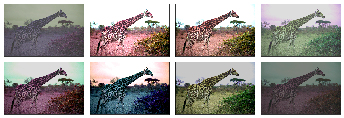
+
### `RandomLighting`
@@ -217,11 +217,11 @@ Use `RandomLighting` for an AlexNet-style PCA-based noise augmentation.
apply(example_image, transforms.RandomLighting(alpha=1))
```
-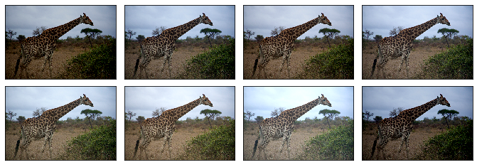
+
-# Composed Augmentations
+## Composed Augmentations
-In practice, we apply multiple augmentation techniques to an image to increase the variety of images in the dataset. Using the `Compose` transform that was introduced in the [Data Transforms tutorial](), we can apply 3 of the transforms we previously used above.
+In practice, we apply multiple augmentation techniques to an image to increase the variety of images in the dataset using the `Compose` transform. We can apply 3 of the transforms we previously used above.
```{.python .input}
@@ -230,6 +230,4 @@ augs = transforms.Compose([
apply(example_image, augs)
```
-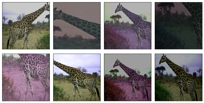
-
-<!-- INSERT SOURCE DOWNLOAD BUTTONS -->
+
diff --git a/docs/python_docs/python/tutorials/packages/gluon/data/datasets.md b/docs/python_docs/python/tutorials/packages/gluon/data/datasets.md
index c09e62a..ecbe121 100644
--- a/docs/python_docs/python/tutorials/packages/gluon/data/datasets.md
+++ b/docs/python_docs/python/tutorials/packages/gluon/data/datasets.md
@@ -18,11 +18,11 @@
# Gluon `Dataset`s and `DataLoader`
-One of the most critical steps for model training and inference is loading the data: without data you can't do Machine Learning! In this tutorial we use the Gluon API to define a [Dataset](/api/python/docs/api/gluon/data/index.html#datasets) and use a [DataLoader](/api/python/docs/api/gluon/data/index.html#dataloader) to iterate through the dataset in mini-batches.
+One of the most critical steps for model training and inference is loading the data: without data you can't do Machine Learning! In this tutorial we use the Gluon API to define a [Dataset](../../../../api/gluon/data/index.rst#datasets) and use a [DataLoader](../../../../api/gluon/data/index.rst#dataloader) to iterate through the dataset in mini-batches.
## Introduction to `Dataset`s
-[Dataset](/api/python/docs/api/gluon/data/index.html#datasets) objects are used to represent collections of data, and include methods to load and parse the data (that is often stored on disk). Gluon has a number of different `Dataset` classes for working with image data straight out-of-the-box, but we'll use the [ArrayDataset](/api/python/docs/api/gluon/data/index.html#mxnet.gluon.data.ArrayDataset) to introduce the idea of a `Dataset`.
+[Dataset](../../../../api/gluon/data/index.rst#datasets) objects are used to represent collections of data, and include methods to load and parse the data (that is often stored on disk). Gluon has a number of different `Dataset` classes for working with image data straight out-of-the-box, but we'll use the [ArrayDataset](../../../../api/gluon/data/index.rst#mxnet.gluon.data.ArrayDataset) to introduce the idea of a `Dataset`.
We first start by generating random data `X` (with 3 variables) and corresponding random labels `y` to simulate a typical supervised learning task. We generate 10 samples and we pass them all to the `ArrayDataset`.
@@ -62,7 +62,7 @@ We get a tuple of a data sample and its corresponding label, which makes sense b
## Introduction to `DataLoader`
-A [DataLoader](/api/python/docs/api/gluon/data/index.html#dataloader) is used to create mini-batches of samples from a [Dataset](/api/python/docs/api/gluon/data/index.html#datasets), and provides a convenient iterator interface for looping these batches. It's typically much more efficient to pass a mini-batch of data through a neural network than a single sample at a time, because the computation can be performed in parallel. A required parameter of `DataLoader` is the size of the mini-b [...]
+A [DataLoader](../../../../api/gluon/data/index.rst#dataloader) is used to create mini-batches of samples from a [Dataset](../../../../api/gluon/data/index.rst#datasets), and provides a convenient iterator interface for looping these batches. It's typically much more efficient to pass a mini-batch of data through a neural network than a single sample at a time, because the computation can be performed in parallel. A required parameter of `DataLoader` is the size of the mini-batches you w [...]
Another benefit of using `DataLoader` is the ability to easily load data in parallel using [multiprocessing](https://docs.python.org/3.6/library/multiprocessing.html). You can set the `num_workers` parameter to the number of CPUs available on your machine for maximum performance, or limit it to a lower number to spare resources.
@@ -90,7 +90,7 @@ Our `data_loader` loop will stop when every sample of `dataset` has been returne
You will often use a few different `Dataset` objects in your Machine Learning project. It's essential to separate your training dataset from testing dataset, and it's also good practice to have validation dataset (a.k.a. development dataset) that can be used for optimising hyperparameters.
-Using Gluon `Dataset` objects, we define the data to be included in each of these separate datasets. Common use cases for loading data are covered already (e.g. [mxnet.gluon.data.vision.datasets.ImageFolderDataset](/api/python/docs/api/gluon/data/vision/index.html)), but it's simple to create your own custom `Dataset` classes for other types of data. You can even use included `Dataset` objects for common datasets if you want to experiment quickly; they download and parse the data for you [...]
+Using Gluon `Dataset` objects, we define the data to be included in each of these separate datasets. Common use cases for loading data are covered already (e.g. [mxnet.gluon.data.vision.datasets.ImageFolderDataset](../../../../api/gluon/data/vision/datasets/index.rst#mxnet.gluon.data.vision.datasets.ImageFolderDataset)), but it's simple to create your own custom `Dataset` classes for other types of data. You can even use included `Dataset` objects for common datasets if you want to exper [...]
Many of the image `Dataset`'s accept a function (via the optional `transform` parameter) which is applied to each sample returned by the `Dataset`. It's useful for performing data augmentation, but can also be used for more simple data type conversion and pixel value scaling as seen below.
@@ -128,12 +128,12 @@ print("Label description: {}".format(label_desc[label]))
`Label description: Bag`<!--notebook-skip-line-->
-<!--notebook-skip-line-->
+<!--notebook-skip-line-->
-When training machine learning models it is important to shuffle the training samples every time you pass through the dataset (i.e. each epoch). Sometimes the order of your samples will have a spurious relationship with the target variable, and shuffling the samples helps remove this. With [DataLoader](/api/python/docs/api/gluon/data/index.html#dataloader) it's as simple as adding `shuffle=True`. You don't need to shuffle the validation and testing data though.
+When training machine learning models it is important to shuffle the training samples every time you pass through the dataset (i.e. each epoch). Sometimes the order of your samples will have a spurious relationship with the target variable, and shuffling the samples helps remove this. With [DataLoader](../../../../api/gluon/data/index.rst#dataloader) it's as simple as adding `shuffle=True`. You don't need to shuffle the validation and testing data though.
-If you have more complex shuffling requirements (e.g. when handling sequential data), take a look at [mxnet.gluon.data.BatchSampler](/api/python/docs/api/gluon/data/index.html#mxnet.gluon.data.BatchSampler) and pass this to your `DataLoader` instead.
+If you have more complex shuffling requirements (e.g. when handling sequential data), take a look at [mxnet.gluon.data.BatchSampler](../../../../api/gluon/data/index.rst#mxnet.gluon.data.BatchSampler) and pass this to your `DataLoader` instead.
```{.python .input}
@@ -210,7 +210,7 @@ for epoch in range(epochs):
# Using own data with included `Dataset`s
-Gluon has a number of different [Dataset](https://mxnet.incubator.apache.org/api/python/gluon/data.html?highlight=dataset#mxnet.gluon.data.Dataset) classes for working with your own image data straight out-of-the-box. You can get started quickly using the [mxnet.gluon.data.vision.datasets.ImageFolderDataset](/api/python/docs/api/gluon/data/vision/datasets/index.html#mxnet.gluon.data.vision.datasets.ImageFolderDataset) which loads images directly from a user-defined folder, and infers the [...]
+Gluon has a number of different [Dataset](../../../../api/gluon/data/index.rst#mxnet.gluon.data.Dataset) classes for working with your own image data straight out-of-the-box. You can get started quickly using the [mxnet.gluon.data.vision.datasets.ImageFolderDataset](../../../../api/gluon/data/vision/datasets/index.rst#mxnet.gluon.data.vision.datasets.ImageFolderDataset) which loads images directly from a user-defined folder, and infers the label (i.e. class) from the folders.
We will run through an example for image classification, but a similar process applies for other vision tasks. If you already have your own collection of images to work with you should partition your data into training and test sets, and place all objects of the same class into seperate folders. Similar to:
```
@@ -241,14 +241,14 @@ if not os.path.isfile(archive_path):
print('Data extracted.')
```
-After downloading and extracting the data archive, we have two folders: `data/101_ObjectCategories` and `data/101_ObjectCategories_test`. We load the data into separate training and testing [ImageFolderDataset](/api/python/docs/api/gluon/data/vision/datasets/index.html#mxnet.gluon.data.vision.datasets.ImageFolderDataset)s.
+After downloading and extracting the data archive, we have two folders: `data/101_ObjectCategories` and `data/101_ObjectCategories_test`. We load the data into separate training and testing [ImageFolderDataset](../../../../api/gluon/data/vision/datasets/index.rst#mxnet.gluon.data.vision.datasets.ImageFolderDataset)s.
```{.python .input}
training_path = os.path.join(data_folder, dataset_name)
testing_path = os.path.join(data_folder, "{}_test".format(dataset_name))
```
-We instantiate the [ImageFolderDataset](https://mxnet.incubator.apache.org/api/python/gluon/data.html?highlight=imagefolderdataset#mxnet.gluon.data.vision.datasets.ImageFolderDataset)s by providing the path to the data, and the folder structure will be traversed to determine which image classes are available and which images correspond to each class. You must take care to ensure the same classes are both the training and testing datasets, otherwise the label encodings can get muddled.
+We instantiate the [ImageFolderDataset](../../../../api/gluon/data/vision/datasets/index.rst#mxnet.gluon.data.vision.datasets.ImageFolderDataset)s by providing the path to the data, and the folder structure will be traversed to determine which image classes are available and which images correspond to each class. You must take care to ensure the same classes are both the training and testing datasets, otherwise the label encodings can get muddled.
Optionally, you can pass a `transform` parameter to these `Dataset`'s as we've seen before.
@@ -260,7 +260,7 @@ test_dataset = mx.gluon.data.vision.datasets.ImageFolderDataset(testing_path)
Samples from these datasets are tuples of data and label. Images are loaded from disk, decoded and optionally transformed when the `__getitem__(i)` method is called (equivalent to `train_dataset[i]`).
-As with the Fashion MNIST dataset the labels will be integer encoded. You can use the `synsets` property of the [ImageFolderDataset](https://mxnet.incubator.apache.org/api/python/gluon/data.html?highlight=imagefolderdataset#mxnet.gluon.data.vision.datasets.ImageFolderDataset)s to retrieve the original descriptions (e.g. `train_dataset.synsets[i]`).
+As with the Fashion MNIST dataset the labels will be integer encoded. You can use the `synsets` property of the [ImageFolderDataset](../../../../api/gluon/data/vision/datasets/index.rst#mxnet.gluon.data.vision.datasets.ImageFolderDataset)s to retrieve the original descriptions (e.g. `train_dataset.synsets[i]`).
```{.python .input}
@@ -283,20 +283,20 @@ assert label == 1
`Label description: Faces_easy` <!--notebook-skip-line-->
-<!--notebook-skip-line-->
+<!--notebook-skip-line-->
# Using own data with custom `Dataset`s
-Sometimes you have data that doesn't quite fit the format expected by the included [Dataset](/api/python/docs/api/gluon/data/index.html#mxnet.gluon.data.Dataset)s. You might be able to preprocess your data to fit the expected format, but it is easy to create your own dataset to do this.
+Sometimes you have data that doesn't quite fit the format expected by the included [Dataset](../../../../api/gluon/data/index.rst#mxnet.gluon.data.Dataset)s. You might be able to preprocess your data to fit the expected format, but it is easy to create your own dataset to do this.
-All you need to do is create a class that implements a `__getitem__` method, that returns a sample (i.e. a tuple of [mx.nd.NDArray](/api/python/docs/api/ndarray/ndarray.html#mxnet.ndarray.NDArray)'s).
+All you need to do is create a class that implements a `__getitem__` method, that returns a sample (i.e. a tuple of [mx.nd.NDArray](../../../../api/legacy/ndarray/ndarray.rst#mxnet.ndarray.NDArray)'s).
# Appendix: Upgrading from Module `DataIter` to Gluon `DataLoader`
-Before Gluon's [DataLoader](/api/python/docs/api/gluon/data/index.html#dataloader), MXNet used [DataIter](/api/python/docs/api/mxnet/io/index.html#mxnet.io.DataIter) objects for loading data for training and testing. `DataIter` has a similar interface for iterating through data, but it isn't directly compatible with typical Gluon `DataLoader` loops. Unlike Gluon `DataLoader` which often returns a tuple of `(data, label)`, a `DataIter` returns a [DataBatch](/api/python/docs/api/mxnet/io/i [...]
+Before Gluon's [DataLoader](../../../../api/gluon/data/index.rst#Dataloader), MXNet used [DataIter](../../../../api/legacy/io/index.rst#mxnet.io.DataIter) objects for loading data for training and testing. `DataIter` has a similar interface for iterating through data, but it isn't directly compatible with typical Gluon `DataLoader` loops. Unlike Gluon `DataLoader` which often returns a tuple of `(data, label)`, a `DataIter` returns a [DataBatch](../../../../api/legacy/io/index.rst#mxnet. [...]
-So you can get up and running with Gluon quicker if you have already implemented complex pre-processing steps using `DataIter`, we have provided a simple class to wrap existing `DataIter` objects so they can be used in a typical Gluon training loop. You can use this class for `DataIter`s such as [mxnet.image.ImageIter](/api/python/docs/api/mxnet/image/index.html#mxnet.image.ImageIter) and [mxnet.io.ImageRecordIter](/api/python/docs/api/mxnet/io/index.html#mxnet.io.ImageDetRecordIter) tha [...]
+So you can get up and running with Gluon quicker if you have already implemented complex pre-processing steps using `DataIter`, we have provided a simple class to wrap existing `DataIter` objects so they can be used in a typical Gluon training loop. You can use this class for `DataIter`s such as [mxnet.image.ImageIter](../../../../api/legacy/image/index.rst#mxnet.image.ImageIter) and [mxnet.io.ImageRecordIter](../../../../api/legacy/io/index.rst#mxnet.io.ImageDetRecordIter) that have sin [...]
```{.python .input}
diff --git a/docs/python_docs/python/tutorials/packages/gluon/image/info_gan.md b/docs/python_docs/python/tutorials/packages/gluon/image/info_gan.md
index d7cd28a..26dcb11 100644
--- a/docs/python_docs/python/tutorials/packages/gluon/image/info_gan.md
+++ b/docs/python_docs/python/tutorials/packages/gluon/image/info_gan.md
@@ -18,8 +18,8 @@
# Image similarity search with InfoGAN
-This notebook shows how to implement an InfoGAN based on Gluon. InfoGAN is an extension of GANs, where the generator input is split in 2 parts: random noise and a latent code (see [InfoGAN Paper](https://arxiv.org/pdf/1606.03657.pdf)).
-The codes are made meaningful by maximizing the mutual information between code and generator output. InfoGAN learns a disentangled representation in a completely unsupervised manner. It can be used for many applications such as image similarity search. This notebook uses the DCGAN example from the [Straight Dope Book](https://gluon.mxnet.io/chapter14_generative-adversarial-networks/dcgan.html) and extends it to create an InfoGAN.
+This notebook shows how to implement an InfoGAN based on Gluon. InfoGAN is an extension of GANs, where the generator input is split in 2 parts: random noise and a latent code (see [InfoGAN Paper](https://arxiv.org/pdf/1606.03657.pdf)).
+The codes are made meaningful by maximizing the mutual information between code and generator output. InfoGAN learns a disentangled representation in a completely unsupervised manner. It can be used for many applications such as image similarity search. This notebook uses the DCGAN example from the [Straight Dope Book](https://gluon.mxnet.io/chapter14_generative-adversarial-networks/dcgan.html) and extends it to create an InfoGAN.
```{.python .input}
@@ -93,7 +93,7 @@ def get_files(data_dir):
img_arr = transform(img_arr)
images.append(img_arr)
filenames.append(path + "/" + fname)
- return images, filenames
+ return images, filenames
```
Load the dataset `lfw_dataset` which contains images of celebrities.
@@ -123,7 +123,7 @@ class Generator(gluon.HybridBlock):
self.prev = nn.HybridSequential()
self.prev.add(nn.Dense(1024, use_bias=False), nn.BatchNorm(), nn.Activation(activation='relu'))
self.G = nn.HybridSequential()
-
+
self.G.add(nn.Conv2DTranspose(64 * 8, 4, 1, 0, use_bias=False))
self.G.add(nn.BatchNorm())
self.G.add(nn.Activation('relu'))
@@ -167,7 +167,7 @@ class Discriminator(gluon.HybridBlock):
self.D.add(nn.LeakyReLU(0.2))
self.D.add(nn.Dense(1024, use_bias=False), nn.BatchNorm(), nn.Activation(activation='relu'))
-
+
self.prob = nn.Dense(1)
self.feat = nn.HybridSequential()
self.feat.add(nn.Dense(128, use_bias=False), nn.BatchNorm(), nn.Activation(activation='relu'))
@@ -182,14 +182,14 @@ class Discriminator(gluon.HybridBlock):
feat = self.feat(x)
category_prob = self.category_prob(feat)
continuous_mean = self.continuous_mean(feat)
-
+
return prob, category_prob, continuous_mean
```
The InfoGAN has the following layout.
<img src="https://raw.githubusercontent.com/dmlc/web-data/master/mxnet/doc/tutorials/info_gan/InfoGAN.png" style="width:800px;height:250px;">
-Discriminator and Generator are the same as in the DCGAN example. On top of the Disciminator is the Q model, which is estimating the code `c` for given fake images. The Generator's input is random noise and the latent code `c`.
+Discriminator and Generator are the same as in the DCGAN example. On top of the Disciminator is the Q model, which is estimating the code `c` for given fake images. The Generator's input is random noise and the latent code `c`.
## Training Loop
Initialize Generator and Discriminator and define correspoing trainer function.
@@ -231,13 +231,13 @@ if os.path.isfile('infogan_d_latest.params') and os.path.isfile('infogan_g_lates
There are 2 differences between InfoGAN and DCGAN: the extra latent code and the Q network to estimate the code.
The latent code is part of the Generator input and it contains mutliple variables (continuous, categorical) that can represent different distributions. In order to make sure that the Generator uses the latent code, mutual information is introduced into the GAN loss term. Mutual information measures how much X is known given Y or vice versa. It is defined as:
-
+
The InfoGAN loss is:
-
+
-where `V(D,G)` is the GAN loss and the mutual information `I(c, G(z, c))` goes in as regularization. The goal is to reach high mutual information, in order to learn meaningful codes for the data.
+where `V(D,G)` is the GAN loss and the mutual information `I(c, G(z, c))` goes in as regularization. The goal is to reach high mutual information, in order to learn meaningful codes for the data.
Define the loss functions. `SoftmaxCrossEntropyLoss` for the categorical code, `L2Loss` for the continious code and `SigmoidBinaryCrossEntropyLoss` for the normal GAN loss.
@@ -254,7 +254,7 @@ This function samples `c`, `z`, and concatenates them to create the generator in
```{.python .input}
def create_generator_input():
-
+
#create random noise
z = nd.random_normal(0, 1, shape=(batch_size, z_dim), ctx=ctx)
label = nd.array(np.random.randint(n_categories, size=batch_size)).as_in_context(ctx)
@@ -265,7 +265,7 @@ def create_generator_input():
return nd.concat(z, c1, c2, dim=1), label, c2
```
-Define the training loop.
+Define the training loop.
1. The discriminator receives `real_data` and `loss1` measures how many real images have been identified as real
2. The discriminator receives `fake_image` from the Generator and `loss1` measures how many fake images have been identified as fake
3. Update Discriminator. Currently, it is updated every second iteration in order to avoid that the Discriminator becomes too strong. You may want to change that.
@@ -275,38 +275,38 @@ Define the training loop.
```{.python .input}
with SummaryWriter(logdir='./logs/') as sw:
-
+
epochs = 1
counter = 0
for epoch in range(epochs):
print("Epoch", epoch)
starttime = time.time()
-
+
d_error_epoch = nd.zeros((1,), ctx=ctx)
g_error_epoch = nd.zeros((1,), ctx=ctx)
-
+
for idx, data in enumerate(train_dataloader):
-
+
#get real data and generator input
- real_data = data.as_in_context(ctx)
+ real_data = data.as_in_context(ctx)
g_input, label, c2 = create_generator_input()
-
+
#Update discriminator: Input real data and fake data
with autograd.record():
output_real,_,_ = discriminator(real_data)
d_error_real = loss1(output_real, real_label)
-
+
# create fake image and input it to discriminator
fake_image = generator(g_input)
output_fake,_,_ = discriminator(fake_image.detach())
d_error_fake = loss1(output_fake, fake_label)
-
+
# total discriminator error
d_error = d_error_real + d_error_fake
d_error_epoch += d_error.mean()
-
+
#Update D every second iteration
if (counter+1) % 2 == 0:
d_error.backward()
@@ -320,7 +320,7 @@ with SummaryWriter(logdir='./logs/') as sw:
g_error.backward()
g_error_epoch += g_error.mean()
-
+
g_trainer.step(batch_size)
q_trainer.step(batch_size)
@@ -332,7 +332,7 @@ with SummaryWriter(logdir='./logs/') as sw:
%(d_error_epoch.asscalar()/count,g_error_epoch.asscalar()/count, count, epoch))
g_input,_,_ = create_generator_input()
-
+
# create some fake image for logging in MXBoard
fake_image = generator(g_input)
@@ -340,7 +340,7 @@ with SummaryWriter(logdir='./logs/') as sw:
sw.add_scalar(tag='Loss_G', value={'test':d_error_epoch.asscalar()/count}, global_step=counter)
sw.add_image(tag='data_image', image=((fake_image[0]+ 1.0) * 127.5).astype(np.uint8) , global_step=counter)
sw.flush()
-
+
discriminator.save_parameters("infogan_d_latest.params")
generator.save_parameters("infogan_g_latest.params")
```
@@ -384,12 +384,12 @@ Take some images from the test data, obtain its feature vector from `discriminat
```{.python .input}
-feature_size = 8192
+feature_size = 8192
features = nd.zeros((len(test_images), feature_size), ctx=ctx)
for idx, image in enumerate(test_images):
-
+
feature = discriminator(nd.array(image, ctx=ctx))
feature = feature.reshape(feature_size,)
features[idx,:] = feature.copyto(ctx)
@@ -407,7 +407,7 @@ for image in test_images[:100]:
plt.subplot(1,10,1)
visualize(image)
- for i in range(2,9):
+ for i in range(2,9):
if indices[i-1][1] < 1.5:
plt.subplot(1,10,i)
sim = test_images[indices[i-1][0]].reshape(3,64,64)
@@ -415,14 +415,14 @@ for image in test_images[:100]:
plt.show()
plt.clf()
```
-<!--notebook-skip-line-->
+<!--notebook-skip-line-->
## How the Generator learns
We trained the Generator for a couple of epochs and stored a couple of fake images per epoch. Check the video.
- 
-
+ 
+
-The following function computes the TSNE on the feature matrix and stores the result in a json-file. This file can be loaded with [TSNEViewer](https://ml4a.github.io/guides/ImageTSNEViewer/)
+The following function computes the TSNE on the feature matrix and stores the result in a json-file. This file can be loaded with [TSNEViewer](https://ml4a.github.io/guides/ImageTSNEViewer/)
```{.python .input}
@@ -437,15 +437,15 @@ tsne = TSNE(n_components=2, learning_rate=150, perplexity=30, verbose=2).fit_tra
data = []
counter = 0
for i,f in enumerate(test_filenames):
-
+
point = [float((tsne[i,k] - np.min(tsne[:,k]))/(np.max(tsne[:,k]) - np.min(tsne[:,k]))) for k in range(2) ]
data.append({"path": os.path.abspath(os.path.join(os.getcwd(),f)), "point": point})
-
+
with open("imagetsne.json", 'w') as outfile:
json.dump(data, outfile)
```
-Load the file with TSNEViewer. You can now inspect whether similiar looking images are grouped nearby or not.
+Load the file with TSNEViewer. You can now inspect whether similiar looking images are grouped nearby or not.
<img src="https://raw.githubusercontent.com/NRauschmayr/web-data/master/mxnet/doc/tutorials/info_gan/tsne.png" style="width:800px;height:600px;">
diff --git a/docs/python_docs/python/tutorials/packages/gluon/image/mnist.md b/docs/python_docs/python/tutorials/packages/gluon/image/mnist.md
index bed7f08..00ff5db 100644
--- a/docs/python_docs/python/tutorials/packages/gluon/image/mnist.md
+++ b/docs/python_docs/python/tutorials/packages/gluon/image/mnist.md
@@ -21,19 +21,17 @@ In this tutorial, we'll give you a step by step walk-through of how to build a h
MNIST is a widely used dataset for the hand-written digit classification task. It consists of 70,000 labeled 28x28 pixel grayscale images of hand-written digits. The dataset is split into 60,000 training images and 10,000 test images. There are 10 classes (one for each of the 10 digits). The task at hand is to train a model using the 60,000 training images and subsequently test its classification accuracy on the 10,000 test images.
-
+
**Figure 1:** Sample images from the MNIST dataset.
-This tutorial uses MXNet's new high-level interface, gluon package to implement MLP using
+This tutorial uses MXNet's new high-level interface, Gluon package to implement MLP using
imperative fashion.
-This is based on the Mnist tutorial with symbolic approach. You can find it [here](https://mxnet.apache.org/api/python/docs/tutorials/packages/gluon/image/mnist.html).
-
## Prerequisites
To complete this tutorial, we need:
-- MXNet. See the instructions for your operating system in [Setup and Installation](https://mxnet.io/get_started).
+- MXNet. See the instructions for your operating system in [Setup and Installation](https://mxnet.apache.org/get_started).
- [Python Requests](http://docs.python-requests.org/en/master/) and [Jupyter Notebook](http://jupyter.org/index.html).
@@ -94,7 +92,7 @@ In an MLP, the outputs of most FC layers are fed into an activation function, wh
The following code declares three fully connected layers with 128, 64 and 10 neurons each.
The last fully connected layer often has its hidden size equal to the number of output classes in the dataset. Furthermore, these FC layers uses ReLU activation for performing an element-wise ReLU transformation on the FC layer output.
-To do this, we will use [Sequential layer](https://mxnet.io/api/python/docs/api/gluon/_autogen/mxnet.gluon.nn.Sequential.html) type. This is simply a linear stack of neural network layers. `nn.Dense` layers are nothing but the fully connected layers we discussed above.
+To do this, we will use [Sequential layer](../../../../api/gluon/nn/index.rst#mxnet.gluon.nn.Sequential) type. This is simply a linear stack of neural network layers. `nn.Dense` layers are nothing but the fully connected layers we discussed above.
```{.python .input}
# define network
@@ -106,13 +104,13 @@ net.add(nn.Dense(10))
#### Initialize parameters and optimizer
-The following source code initializes all parameters received from parameter dict using [Xavier](https://mxnet.io/api/python/docs/api/gluon-related/_autogen/mxnet.initializer.Xavier.html) initializer
+The following source code initializes all parameters received from parameter dict using [Xavier](../../../../api/initializer/index.rst#mxnet.initializer.Xavier) initializer
to train the MLP network we defined above.
For our training, we will make use of the stochastic gradient descent (SGD) optimizer. In particular, we'll be using mini-batch SGD. Standard SGD processes train data one example at a time. In practice, this is very slow and one can speed up the process by processing examples in small batches. In this case, our batch size will be 100, which is a reasonable choice. Another parameter we select here is the learning rate, which controls the step size the optimizer takes in search of a soluti [...]
-We will use [Trainer](/api/python/docs/api/gluon/trainer.html) class to apply the
-[SGD optimizer](/api/python/docs/api/optimizer/index.html#mxnet.optimizer.SGD) on the
+We will use [Trainer](../../../../api/gluon/trainer.rst) class to apply the
+[SGD optimizer](../../../../api/optimizer/index.rst#mxnet.optimizer.SGD) on the
initialized parameters.
```{.python .input}
@@ -128,7 +126,7 @@ Typically, one runs the training until convergence, which means that we have lea
We will take following steps for training:
-- Define [Accuracy evaluation metric](https://mxnet.io/api/python/metric/metric.html#mxnet.metric.Accuracy) over training data.
+- Define [Accuracy evaluation metric](../../../../api/gluon/metric/index.rst#mxnet.gluon.metric.Accuracy) over training data.
- Loop over inputs for every epoch.
- Forward input through network to get output.
- Compute loss with output and label inside record scope.
@@ -137,7 +135,7 @@ We will take following steps for training:
Loss function takes (output, label) pairs and computes a scalar loss for each sample in the mini-batch. The scalars measure how far each output is from the label.
There are many predefined loss functions in gluon.loss. Here we use
-[softmax_cross_entropy_loss](https://mxnet.io/api/python/gluon/gluon.html#mxnet.gluon.loss.softmax_cross_entropy_loss) for digit classification. We will compute loss and do backward propagation inside
+[softmax_cross_entropy_loss](../../../../api/gluon/loss/index.rst#mxnet.gluon.loss.SoftmaxCrossEntropyLoss) for digit classification. We will compute loss and do backward propagation inside
training scope which is defined by `autograd.record()`.
```{.python .input}
@@ -252,7 +250,7 @@ Now, We will create the network as follows:
net = Net()
```
-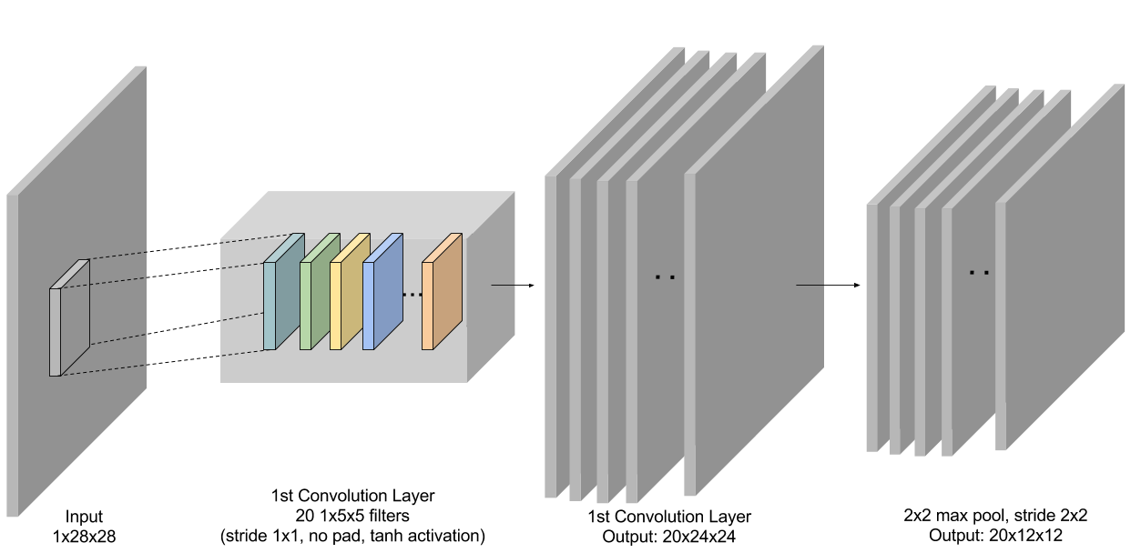{ width=500px }
+{ width=500px }
**Figure 3:** First conv + pooling layer in LeNet.
diff --git a/docs/python_docs/python/tutorials/packages/gluon/loss/custom-loss.md b/docs/python_docs/python/tutorials/packages/gluon/loss/custom-loss.md
index 6aa556f..21e545d 100644
--- a/docs/python_docs/python/tutorials/packages/gluon/loss/custom-loss.md
+++ b/docs/python_docs/python/tutorials/packages/gluon/loss/custom-loss.md
@@ -19,9 +19,9 @@
All neural networks need a loss function for training. A loss function is a quantitive measure of how bad the predictions of the network are when compared to ground truth labels. Given this score, a network can improve by iteratively updating its weights to minimise this loss. Some tasks use a combination of multiple loss functions, but often you'll just use one. MXNet Gluon provides a number of the most commonly used loss functions, and you'll choose certain functions depending on your [...]
-- Regression: [L1Loss](/api/python/docs/api/gluon/loss/index.html#mxnet.gluon.loss.L1Loss), [L2Loss](/api/python/docs/api/gluon/loss/index.html#mxnet.gluon.loss.L2Loss)
-- Classification: [SigmoidBinaryCrossEntropyLoss](/api/python/docs/api/gluon/loss/index.html#mxnet.gluon.loss.SigmoidBinaryCrossEntropyLoss), [SoftmaxBinaryCrossEntropyLoss](/api/python/docs/api/gluon/loss/index.html#mxnet.gluon.loss.SoftmaxBinaryCrossEntropyLoss)
-- Embeddings: [HingeLoss](/api/python/docs/api/gluon/loss/index.html#mxnet.gluon.loss.HingeLoss)
+- Regression: [L1Loss](../../../../api/gluon/loss/index.rst#mxnet.gluon.loss.L1Loss), [L2Loss](../../../../api/gluon/loss/index.rst#mxnet.gluon.loss.L2Loss)
+- Classification: [SigmoidBinaryCrossEntropyLoss](../../../../api/gluon/loss/index.rst#mxnet.gluon.loss.SigmoidBinaryCrossEntropyLoss), [SoftmaxCrossEntropyLoss](../../../../api/gluon/loss/index.rst#mxnet.gluon.loss.SoftmaxCrossEntropyLoss)
+- Embeddings: [HingeLoss](../../../../api/gluon/loss/index.rst#mxnet.gluon.loss.HingeLoss)
However, we may sometimes want to solve problems that require customized loss functions; this tutorial shows how we can do that in Gluon. We will implement contrastive loss which is typically used in Siamese networks.
@@ -37,7 +37,7 @@ import random
[Contrastive loss](http://yann.lecun.com/exdb/publis/pdf/hadsell-chopra-lecun-06.pdf) is a distance-based loss function. During training, pairs of images are fed into a model. If the images are similar, the loss function will return 0, otherwise 1.
-<img src="images/contrastive_loss.jpeg" width="400">
+
*Y* is a binary label indicating similarity between training images. Contrastive loss uses the Euclidean distance *D* between images and is the sum of 2 terms:
- the loss for a pair of similar points
@@ -45,7 +45,7 @@ import random
The loss function uses a margin *m* which is has the effect that dissimlar pairs only contribute if their loss is within a certain margin.
-In order to implement such a customized loss function in Gluon, we only need to define a new class that is inheriting from the [Loss](/api/python/docs/api/gluon/loss/index.html#mxnet.gluon.loss.Loss) base class. We then define the contrastive loss logic in the [hybrid_forward](/api/python/docs/api/gluon/hybrid_block.html#mxnet.gluon.HybridBlock.hybrid_forward) method. This method takes the images `image1`, `image2` and the label which defines whether `image1` and `image2` are similar (= [...]
+In order to implement such a customized loss function in Gluon, we only need to define a new class that is inheriting from the [Loss](../../../../api/gluon/loss/index.rst#mxnet.gluon.loss.Loss) base class. We then define the contrastive loss logic in the [hybrid_forward](../../../../api/gluon/hybrid_block.rst#mxnet.gluon.HybridBlock.hybrid_forward) method. This method takes the images `image1`, `image2` and the label which defines whether `image1` and `image2` are similar (=0) or dissi [...]
```{.python .input}
@@ -156,7 +156,7 @@ plt.show()
```
-
+
### Train the Siamese network
@@ -208,7 +208,7 @@ for i, data in enumerate(test_dataloader):
```
-
+
### Common pitfalls with custom loss functions
diff --git a/docs/python_docs/python/tutorials/packages/gluon/loss/kl_divergence.md b/docs/python_docs/python/tutorials/packages/gluon/loss/kl_divergence.md
index 7eb6f76..86047d7 100644
--- a/docs/python_docs/python/tutorials/packages/gluon/loss/kl_divergence.md
+++ b/docs/python_docs/python/tutorials/packages/gluon/loss/kl_divergence.md
@@ -19,7 +19,7 @@
Kullback-Leibler (KL) Divergence is a measure of how one probability distribution is different from a second, reference probability distribution. Smaller KL Divergence values indicate more similar distributions and, since this loss function is differentiable, we can use gradient descent to minimize the KL divergence between network outputs and some target distribution. As an example, this can be used in Variational Autoencoders (VAEs), and reinforcement learning policy networks such as [ [...]
-In MXNet Gluon, we can use [KLDivLoss](/api/python/docs/api/gluon/_autogen/mxnet.gluon.loss.KLDivLoss.html) to compare categorical distributions. One important thing to note is that the KL Divergence is an asymmetric measure (i.e. `KL(P,Q) != KL(Q,P)`): order matters and we should compare our predicted distribution with our target distribution in that order. Another thing to note is that there are two ways to use [KLDivLoss](/api/python/docs/api/gluon/_autogen/mxnet.gluon.loss.KLDivLoss. [...]
+In MXNet Gluon, we can use [KLDivLoss](../../../../api/gluon/loss/index.rst#mxnet.gluon.loss.KLDivLoss) to compare categorical distributions. One important thing to note is that the KL Divergence is an asymmetric measure (i.e. `KL(P,Q) != KL(Q,P)`): order matters and we should compare our predicted distribution with our target distribution in that order. Another thing to note is that there are two ways to use [KLDivLoss](../../../../api/gluon/loss/index.rst#mxnet.gluon.loss.KLDivLoss) th [...]
As an example, let's compare a few categorical distributions (`dist_1`, `dist_2` and `dist_3`), each with 4 categories.
@@ -46,14 +46,14 @@ plt.bar(idx, dist_3, alpha=0.5, color='aqua')
plt.title('Distributions 1 & 3')
```
-We can see visually that distributions 1 and 2 are more similar than distributions 1 and 3. We'll confirm this result using [KLDivLoss](/api/python/docs/api/gluon/_autogen/mxnet.gluon.loss.KLDivLoss.html). When using [KLDivLoss](/api/python/docs/api/gluon/_autogen/mxnet.gluon.loss.KLDivLoss.html) with the default `from_logits=True` we need:
+We can see visually that distributions 1 and 2 are more similar than distributions 1 and 3. We'll confirm this result using [KLDivLoss](../../../../api/gluon/loss/index.rst#mxnet.gluon.loss.KLDivLoss). When using [KLDivLoss](../../../../api/gluon/loss/index.rst#mxnet.gluon.loss.KLDivLoss) with the default `from_logits=True` we need:
1. our predictions to be parameters of a logged probability distribution.
2. our targets to be parameters of a probability distribution (i.e. not logged).
-We often apply a [softmax](/api/python/docs/api/ndarray/_autogen/mxnet.ndarray.softmax.html) operation to the output of our network to get a distribution, but this can have a numerically unstable gradient calculation. As as stable alternative, we use [log_softmax](/api/python/docs/api/ndarray/_autogen/mxnet.ndarray.log_softmax.html) and so this is what is expected by [KLDivLoss](/api/python/docs/api/gluon/_autogen/mxnet.gluon.loss.KLDivLoss.html) when `from_logits=True`. We also usually [...]
+We often apply a [softmax](../../../../api/npx/generated/mxnet.npx.softmax.rst) operation to the output of our network to get a distribution, but this can have a numerically unstable gradient calculation. As as stable alternative, we use [log_softmax](../../../../api/npx/generated/mxnet.npx.log_softmax.rst) and so this is what is expected by [KLDivLoss](../../../../api/gluon/loss/index.rst#mxnet.gluon.loss.KLDivLoss) when `from_logits=True`. We also usually work with batches of predictio [...]
-Since we're already working with distributions in this example, we don't need to apply the softmax and only need to apply [log](/api/python/docs/api/ndarray/_autogen/mxnet.ndarray.log.html). And we'll create batch dimensions even though we're working with single distributions.
+Since we're already working with distributions in this example, we don't need to apply the softmax and only need to apply [log](../../../../api/np/generated/mxnet.np.log.rst). And we'll create batch dimensions even though we're working with single distributions.
```
def kl_divergence(dist_a, dist_b):
@@ -81,13 +81,13 @@ As expected we see a smaller KL Divergence for distributions 1 & 2 than 1 & 3. A
#### `from_logits=False`
-Alternatively, instead of manually applying the [log_softmax](/api/python/docs/api/ndarray/_autogen/mxnet.ndarray.log_softmax.html) to our network outputs, we can leave that to the loss function. When setting `from_logits=False` on [KLDivLoss](/api/python/docs/api/gluon/_autogen/mxnet.gluon.loss.KLDivLoss.html), the [log_softmax](/api/python/docs/api/ndarray/_autogen/mxnet.ndarray.log_softmax.html) is applied to the first argument passed to `loss_fn`. As an example, let's assume our netw [...]
+Alternatively, instead of manually applying the [log_softmax](../../../../api/npx/generated/mxnet.npx.log_softmax.rst) to our network outputs, we can leave that to the loss function. When setting `from_logits=False` on [KLDivLoss](../../../../api/gluon/loss/index.rst#mxnet.gluon.loss.KLDivLoss), the [log_softmax](../../../../api/npx/generated/mxnet.npx.log_softmax.rst) is applied to the first argument passed to `loss_fn`. As an example, let's assume our network outputs us the values belo [...]
```
output = mx.nd.array([0.39056206, 1.3068528, 0.39056206, -0.30258512])
```
-We can pass this to our [KLDivLoss](/api/python/docs/api/gluon/_autogen/mxnet.gluon.loss.KLDivLoss.html) loss function (with `from_logits=False`) and get the same KL Divergence between `dist_1` and `dist_2` as before, because the [log_softmax](/api/python/docs/api/ndarray/_autogen/mxnet.ndarray.log_softmax.html) is applied within the loss function.
+We can pass this to our [KLDivLoss](../../../../api/gluon/loss/index.rst#mxnet.gluon.loss.KLDivLoss) loss function (with `from_logits=False`) and get the same KL Divergence between `dist_1` and `dist_2` as before, because the [log_softmax](../../../../api/npx/generated/mxnet.npx.log_softmax.rst) is applied within the loss function.
```
def kl_divergence_not_from_logits(dist_a, dist_b):
@@ -107,7 +107,7 @@ print("Distribution 1 compared with Distribution 2: {}".format(
### Advanced: Common Support
-Occasionally, you might have issues with [KLDivLoss](/api/python/docs/api/gluon/_autogen/mxnet.gluon.loss.KLDivLoss.html). One common issue arises when the support of the distributions being compared are not the same. 'Support' here is referring to the values of the distribution which have a non-zero probability. Conveniently, all our examples above had the same support, but we might have a case where some categories have a probability of 0.
+Occasionally, you might have issues with [KLDivLoss](../../../../api/gluon/loss/index.rst#mxnet.gluon.loss.KLDivLoss). One common issue arises when the support of the distributions being compared are not the same. 'Support' here is referring to the values of the distribution which have a non-zero probability. Conveniently, all our examples above had the same support, but we might have a case where some categories have a probability of 0.
```
@@ -123,7 +123,7 @@ We can see that the result is `nan`, which will obviously cause issues when calc
### Advanced: Aggregation
-One minor difference between the true definition of KL Divergence and the result from [KLDivLoss](/api/python/docs/api/gluon/_autogen/mxnet.gluon.loss.KLDivLoss.html) is how the aggregation of category contributions is performed. Although the true definition sums up these contributions, the default behaviour in MXNet Gluon is to average terms along the batch dimension. As a result, the [KLDivLoss](/api/python/docs/api/gluon/_autogen/mxnet.gluon.loss.KLDivLoss.html) output will be smaller [...]
+One minor difference between the true definition of KL Divergence and the result from [KLDivLoss](../../../../api/gluon/loss/index.rst#mxnet.gluon.loss.KLDivLoss) is how the aggregation of category contributions is performed. Although the true definition sums up these contributions, the default behaviour in MXNet Gluon is to average terms along the batch dimension. As a result, the [KLDivLoss](../../../../api/gluon/loss/index.rst#mxnet.gluon.loss.KLDivLoss) output will be smaller than th [...]
```
true_divergence = (dist_2*(np.log(dist_2)-np.log(dist_1))).sum()
diff --git a/docs/python_docs/python/tutorials/packages/gluon/loss/loss.md b/docs/python_docs/python/tutorials/packages/gluon/loss/loss.md
index e7efbcad..a94c5c0 100644
--- a/docs/python_docs/python/tutorials/packages/gluon/loss/loss.md
+++ b/docs/python_docs/python/tutorials/packages/gluon/loss/loss.md
@@ -19,9 +19,9 @@
Loss functions are used to train neural networks and to compute the difference between output and target variable. A critical component of training neural networks is the loss function. A loss function is a quantative measure of how bad the predictions of the network are when compared to ground truth labels. Given this score, a network can improve by iteratively updating its weights to minimise this loss. Some tasks use a combination of multiple loss functions, but often you'll just use [...]
-- regression: [L1Loss](/api/python/docs/api/gluon/loss/index.html#mxnet.gluon.loss.L1Loss), [L2Loss](/api/python/docs/api/gluon/loss/index.html#mxnet.gluon.loss.L2Loss)
-- classification: [SigmoidBinaryCrossEntropyLoss](/api/python/docs/api/gluon/loss/index.html#mxnet.gluon.loss.SigmoidBinaryCrossEntropyLoss), [SoftmaxCrossEntropyLoss](/api/python/docs/api/gluon/loss/index.html#mxnet.gluon.loss.SoftmaxCrossEntropyLoss)
-- embeddings: [HingeLoss](/api/python/docs/api/gluon/_autogen/mxnet.gluon.loss.HingeLoss.html)
+- Regression: [L1Loss](../../../../api/gluon/loss/index.rst#mxnet.gluon.loss.L1Loss), [L2Loss](../../../../api/gluon/loss/index.rst#mxnet.gluon.loss.L2Loss)
+- Classification: [SigmoidBinaryCrossEntropyLoss](../../../../api/gluon/loss/index.rst#mxnet.gluon.loss.SigmoidBinaryCrossEntropyLoss), [SoftmaxCrossEntropyLoss](../../../../api/gluon/loss/index.rst#mxnet.gluon.loss.SoftmaxCrossEntropyLoss)
+- Embeddings: [HingeLoss](../../../../api/gluon/loss/index.rst#mxnet.gluon.loss.HingeLoss)
We'll first import the modules, where the `mxnet.gluon.loss` module is imported as `gloss` to avoid the commonly used name `loss`.
@@ -103,7 +103,7 @@ def show_classification_loss(loss):
plot(x, y)
```
-#### [L1 Loss](https://mxnet.apache.org/api/python/gluon/loss.html#mxnet.gluon.loss.L1Loss)
+#### [L1 Loss](../../../../api/gluon/loss/index.rst#mxnet.gluon.loss.L1Loss)
L1 Loss, also called Mean Absolute Error, computes the sum of absolute distance between target values and the output of the neural network. It is defined as:
@@ -115,7 +115,7 @@ It is a non-smooth function that can lead to non-convergence. It creates the sam
show_regression_loss(gloss.L1Loss())
```
-#### [L2 Loss](https://mxnet.apache.org/api/python/gluon/loss.html#mxnet.gluon.loss.L2Loss)
+#### [L2 Loss](../../../../api/gluon/loss/index.rst#mxnet.gluon.loss.L2Loss)
L2Loss, also called Mean Squared Error, is a regression loss function that computes the squared distances between the target values and the output of the neural network. It is defined as:
@@ -127,7 +127,7 @@ Compared to L1, L2 loss it is a smooth function and it creates larger gradients
show_regression_loss(gloss.L2Loss())
```
-#### [Huber Loss](https://mxnet.apache.org/api/python/gluon/loss.html#mxnet.gluon.loss.HuberLosss)
+#### [Huber Loss](../../../../api/gluon/loss/index.rst#mxnet.gluon.loss.HuberLoss)
HuberLoss combines advantages of L1 and L2 loss. It calculates a smoothed L1 loss that is equal to L1 if the absolute error exceeds a threshold $$\rho$$, otherwise it is equal to L2. It is defined as:
$$
@@ -144,7 +144,7 @@ show_regression_loss(gloss.HuberLoss(rho=1))
An example of where Huber Loss is used can be found in [Deep Q Network](https://openai.com/blog/openai-baselines-dqn/).
-#### [Cross Entropy Loss with Sigmoid](https://mxnet.apache.org/api/python/gluon/loss.html#mxnet.gluon.loss.SigmoidBinaryCrossEntropyLoss)
+#### [Cross Entropy Loss with Sigmoid](../../../../api/gluon/loss/index.rst#mxnet.gluon.loss.SigmoidBinaryCrossEntropyLoss)
Binary Cross Entropy is a loss function used for binary classification problems e.g. classifying images into 2 classes. Cross entropy measures the difference between two probability distributions and it is defined as:
$$\sum_i -{(y\log(p) + (1 - y)\log(1 - p))} $$
@@ -154,7 +154,7 @@ Before the loss is computed a sigmoid activation is applied per default. If your
show_classification_loss(gloss.SigmoidBinaryCrossEntropyLoss())
```
-#### [Cross Entropy Loss with Softmax](https://mxnet.apache.org/api/python/gluon/loss.html#mxnet.gluon.loss.SoftmaxCrossEntropyLoss)
+#### [Cross Entropy Loss with Softmax](../../../../api/gluon/loss/index.rst#mxnet.gluon.loss.SoftmaxCrossEntropyLoss)
In classification, we often apply the
softmax operator to the predicted outputs to obtain prediction probabilities,
@@ -172,7 +172,7 @@ y = nd.array([0, 1])
loss(x, y)
```
-#### [Hinge Loss](https://mxnet.apache.org/api/python/gluon/loss.html#mxnet.gluon.loss.HingeLoss)
+#### [Hinge Loss](../../../../api/gluon/loss/index.rst#mxnet.gluon.loss.HingeLoss)
Commonly used in Support Vector Machines (SVMs), Hinge Loss is used to additionally penalize predictions that are correct but fall within a margin between classes (the region around a decision boundary). Unlike `SoftmaxCrossEntropyLoss`, it's rarely used for neural network training. It is defined as:
@@ -184,7 +184,7 @@ $$
show_classification_loss(gloss.HingeLoss())
```
-#### [Logistic Loss](/api/python/docs/api/gluon/loss/index.html#mxnet.gluon.loss.LogisticLoss)
+#### [Logistic Loss](../../../../api/gluon/loss/index.rst#mxnet.gluon.loss.LogisticLoss)
The Logistic Loss function computes the performance of binary classification models.
$$
@@ -196,7 +196,7 @@ The log loss decreases the closer the prediction is to the actual label. It is s
show_classification_loss(gloss.LogisticLoss())
```
-#### [Kullback-Leibler Divergence Loss](/api/python/docs/api/gluon/loss/index.html#mxnet.gluon.loss.KLDivLoss)
+#### [Kullback-Leibler Divergence Loss](../../../../api/gluon/loss/index.rst#mxnet.gluon.loss.KLDivLoss)
The Kullback-Leibler divergence loss measures the divergence between two probability distributions by calculating the difference between cross entropy and entropy. It takes as input the probability of predicted label and the probability of true label.
@@ -218,7 +218,7 @@ loss = loss_fn(output, target_dist)
print('loss (kl divergence): {}'.format(loss.asnumpy().tolist()))
```
-#### [Triplet Loss](/api/python/docs/api/gluon/loss/index.html#mxnet.gluon.loss.TripletLoss)
+#### [Triplet Loss](../../../../api/gluon/loss/index.rst#mxnet.gluon.loss.TripletLoss)
Triplet loss takes three input arrays and measures the relative similarity. It takes a positive and negative input and the anchor.
@@ -230,17 +230,17 @@ $$
The loss function minimizes the distance between similar inputs and maximizes the distance between dissimilar ones.
In the case of learning embeddings for images of characters, the network may get as input the following 3 images:
-
+
The network would learn to minimize the distance between the two `A`'s and maximize the distance between `A` and `Z`.
-#### [CTC Loss](/api/python/docs/api/gluon/loss/index.html#mxnet.gluon.loss.CTCLoss)
+#### [CTC Loss](../../../../api/gluon/loss/index.rst#mxnet.gluon.loss.CTCLoss)
CTC Loss is the [connectionist temporal classification loss](https://distill.pub/2017/ctc/) . It is used to train recurrent neural networks with variable time dimension. It learns the alignment and labelling of input sequences. It takes a sequence as input and gives probabilities for each timestep. For instance, in the following image the word is not well aligned with the 5 timesteps because of the different sizes of characters. CTC Loss finds for each timestep the highest probability e. [...]
-
+
-#### [Cosine Embedding Loss](/api/python/docs/api/gluon/loss/index.html#mxnet.gluon.loss.CosineEmbeddingLoss)
+#### [Cosine Embedding Loss](../../../../api/gluon/loss/index.rst#mxnet.gluon.loss.CosineEmbeddingLoss)
The cosine embedding loss computes the cosine distance between two input vectors.
$$
@@ -270,7 +270,7 @@ loss = gloss.CosineEmbeddingLoss()
print(loss(x,y,label))
```
-#### [PoissonNLLLoss](/api/python/docs/api/gluon/loss/index.html#mxnet.gluon.loss.PoissonNLLLoss)
+#### [PoissonNLLLoss](../../../../api/gluon/loss/index.rst#mxnet.gluon.loss.PoissonNLLLoss)
Poisson distribution is widely used for modelling count data. It is defined as:
$$
diff --git a/docs/python_docs/python/tutorials/packages/gluon/training/fit_api_tutorial.md b/docs/python_docs/python/tutorials/packages/gluon/training/fit_api_tutorial.md
index ce270da..06592aa 100644
--- a/docs/python_docs/python/tutorials/packages/gluon/training/fit_api_tutorial.md
+++ b/docs/python_docs/python/tutorials/packages/gluon/training/fit_api_tutorial.md
@@ -17,7 +17,7 @@
# MXNet Gluon Fit API
-In this tutorial, you will learn how to use the [Gluon Fit API](https://cwiki.apache.org/confluence/display/MXNET/Gluon+Fit+API+-+Tech+Design) which is the easiest way to train deep learning models using the [Gluon API](/api/python/docs/tutorials/packages/gluon/index.html) in Apache MXNet.
+In this tutorial, you will learn how to use the [Gluon Fit API](https://cwiki.apache.org/confluence/display/MXNET/Gluon+Fit+API+-+Tech+Design) which is the easiest way to train deep learning models using the [Gluon API](../index.rst) in Apache MXNet.
With the Fit API, you can train a deep learning model with a minimal amount of code. Just specify the network, loss function and the data you want to train on. You don't need to worry about the boiler plate code to loop through the dataset in batches (often called as 'training loop'). Advanced users can train with bespoke training loops, and many of these use cases will be covered by the Fit API.
@@ -27,7 +27,7 @@ To demonstrate the Fit API, you will train an image classification model using t
To complete this tutorial, you will need:
-- [MXNet](/get_started) (The version of MXNet will be >= 1.5.0, you can use `pip install mxnet` to get 1.5.0 release pip package or build from source with master, refer to [MXNet installation](/get_started?version=master&platform=linux&language=python&environ=pip&processor=cpu)
+- [MXNet](https://mxnet.apache.org/get_started) (The version of MXNet will be >= 1.5.0, you can use `pip install mxnet` to get 1.5.0 release pip package or build from source with master, refer to [MXNet installation](https://mxnet.apache.org/get_started?version=master&platform=linux&language=python&environ=pip&processor=cpu)
- [Jupyter Notebook](https://jupyter.org/index.html) (For interactively running the provided .ipynb file)
@@ -89,7 +89,7 @@ val_data_loader = gluon.data.DataLoader(fashion_mnist_val, batch_size=batch_size
## Model and Optimizers
-Let's load the resnet-18 model architecture from [Gluon Model Zoo](https://mxnet.apache.org/api/python/gluon/model_zoo.html) and initialize its parameters. The Gluon Model Zoo contains a repository of pre-trained models as well the model architecture definitions. We are using the model architecture from the model zoo in order to train it from scratch.
+Let's load the resnet-18 model architecture from [Gluon Model Zoo](../../../../api/gluon/model_zoo/index.rst) and initialize its parameters. The Gluon Model Zoo contains a repository of pre-trained models as well the model architecture definitions. We are using the model architecture from the model zoo in order to train it from scratch.
```{.python .input}
@@ -98,7 +98,7 @@ resnet_18_v1.initialize(init = mx.init.Xavier(), ctx=ctx)
```
We will be using `SoftmaxCrossEntropyLoss` as the loss function since this is a multi-class classification problem. We will be using `sgd` (Stochastic Gradient Descent) as the optimizer.
-You can experiment with a [different loss](/api/python/docs/api/gluon/loss/index.html) or [optimizer](/api/python/docs/api/optimizer/index.html) as well.
+You can experiment with a [different loss](../../../../api/gluon/loss/index.rst) or [optimizer](../../../../api/optimizer/index.rst) as well.
```{.python .input}
@@ -252,7 +252,7 @@ with warnings.catch_warnings():
Epoch 2, loss 0.3229 <!--notebook-skip-line-->
```
-You can load the saved model, by using the `load_parameters` API in Gluon. For more details refer to the [Loading model parameters from file tutorial](/api/python/docs/tutorials/packages/gluon/blocks/save_load_params.html#saving-model-parameters-to-file)
+You can load the saved model, by using the `load_parameters` API in Gluon. For more details refer to the [Loading model parameters from file tutorial](../blocks/save_load_params.ipynb#Loading-model-parameters-from-file)
```{.python .input}
diff --git a/docs/python_docs/python/tutorials/packages/gluon/training/learning_rates/learning_rate_finder.md b/docs/python_docs/python/tutorials/packages/gluon/training/learning_rates/learning_rate_finder.md
index 0cab619..b43358c 100644
--- a/docs/python_docs/python/tutorials/packages/gluon/training/learning_rates/learning_rate_finder.md
+++ b/docs/python_docs/python/tutorials/packages/gluon/training/learning_rates/learning_rate_finder.md
@@ -20,7 +20,7 @@
Setting the learning rate for stochastic gradient descent (SGD) is crucially important when training neural network because it controls both the speed of convergence and the ultimate performance of the network. Set the learning too low and you could be twiddling your thumbs for quite some time as the parameters update very slowly. Set it too high and the updates will skip over optimal solutions, or worse the optimizer might not converge at all!
-Leslie Smith from the U.S. Naval Research Laboratory presented a method for finding a good learning rate in a paper called ["Cyclical Learning Rates for Training Neural Networks"](https://arxiv.org/abs/1506.01186). We implement this method in MXNet (with the Gluon API) and create a 'Learning Rate Finder' which you can use while training your own networks. We take a look at the central idea of the paper, cyclical learning rate schedules, in the ['Advanced Learning Rate Schedules'](/api/py [...]
+Leslie Smith from the U.S. Naval Research Laboratory presented a method for finding a good learning rate in a paper called ["Cyclical Learning Rates for Training Neural Networks"](https://arxiv.org/abs/1506.01186). We implement this method in MXNet (with the Gluon API) and create a 'Learning Rate Finder' which you can use while training your own networks. We take a look at the central idea of the paper, cyclical learning rate schedules, in the ['Advanced Learning Rate Schedules'](./learn [...]
## Simple Idea
@@ -327,6 +327,6 @@ Although we get quite similar results to when we set the learning rate at 0.05 (
## Wrap Up
-Give Learning Rate Finder a try on your current projects, and experiment with the different learning rate schedules found in the [basic learning rate tutorial](/api/python/docs/tutorials/packages/gluon/training/learning_rates/learning_rate_schedules.html) and the [advanced learning rate tutorial](/api/python/docs/tutorials/packages/gluon/training/learning_rates/learning_rate_schedules_advanced.html).
+Give Learning Rate Finder a try on your current projects, and experiment with the different learning rate schedules found in the [basic learning rate tutorial](./learning_rate_schedules.ipynb) and the [advanced learning rate tutorial](./learning_rate_schedules_advanced.ipynb).
<!-- INSERT SOURCE DOWNLOAD BUTTONS -->
diff --git a/docs/python_docs/python/tutorials/packages/gluon/training/learning_rates/learning_rate_schedules.md b/docs/python_docs/python/tutorials/packages/gluon/training/learning_rates/learning_rate_schedules.md
index e26218a..2a9ca0d 100644
--- a/docs/python_docs/python/tutorials/packages/gluon/training/learning_rates/learning_rate_schedules.md
+++ b/docs/python_docs/python/tutorials/packages/gluon/training/learning_rates/learning_rate_schedules.md
@@ -66,7 +66,7 @@ plot_schedule(schedule)
```
-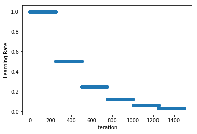 <!--notebook-skip-line-->
+ <!--notebook-skip-line-->
Note: the `base_lr` is used to determine the initial learning rate. It takes a default value of 0.01 since we inherit from `mx.lr_scheduler.LRScheduler`, but it can be set as a property of the schedule. We will see later in this tutorial that `base_lr` is set automatically when providing the `lr_schedule` to `Optimizer`. Also be aware that the schedules in `mx.lr_scheduler` have state (i.e. counters, etc) so calling the schedule out of order may give unexpected results.
@@ -81,7 +81,7 @@ plot_schedule(schedule)
```
-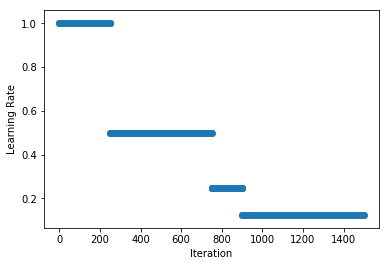 <!--notebook-skip-line-->
+ <!--notebook-skip-line-->
### Polynomial Schedule
@@ -95,7 +95,7 @@ plot_schedule(schedule)
```
-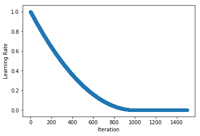 <!--notebook-skip-line-->
+ <!--notebook-skip-line-->
Note: unlike `FactorScheduler`, the `base_lr` is set as an argument when instantiating the schedule.
@@ -113,7 +113,7 @@ class CosineAnnealingSchedule():
self.min_lr = min_lr
self.max_lr = max_lr
self.cycle_length = cycle_length
-
+
def __call__(self, iteration):
if iteration <= self.cycle_length:
unit_cycle = (1 + math.cos(iteration * math.pi / self.cycle_length)) / 2
@@ -128,12 +128,12 @@ plot_schedule(schedule)
```
-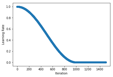 <!--notebook-skip-line-->
+ <!--notebook-skip-line-->
## Using Schedules
-While training a simple handwritten digit classifier on the MNIST dataset, we take a look at how to use a learning rate schedule during training. Our demonstration model is a basic convolutional neural network. We start by preparing our `DataLoader` and defining the network.
+While training a simple handwritten digit classifier on the MNIST dataset, we take a look at how to use a learning rate schedule during training. Our demonstration model is a basic convolutional neural network. We start by preparing our `DataLoader` and defining the network.
As discussed above, the schedule should return a learning rate given an (1-based) iteration index.
@@ -169,7 +169,7 @@ def build_cnn():
# Second fully connected layer with as many neurons as the number of classes
net.add(nn.Dense(num_outputs))
return net
-
+
net = build_cnn()
```
diff --git a/docs/python_docs/python/tutorials/packages/gluon/training/learning_rates/learning_rate_schedules_advanced.md b/docs/python_docs/python/tutorials/packages/gluon/training/learning_rates/learning_rate_schedules_advanced.md
index e6c40cd..778a616 100644
--- a/docs/python_docs/python/tutorials/packages/gluon/training/learning_rates/learning_rate_schedules_advanced.md
+++ b/docs/python_docs/python/tutorials/packages/gluon/training/learning_rates/learning_rate_schedules_advanced.md
@@ -88,7 +88,7 @@ plot_schedule(schedule)
```
-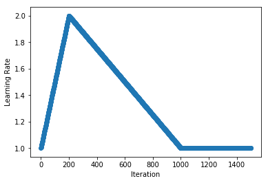 <!--notebook-skip-line-->
+ <!--notebook-skip-line-->
### Cosine
@@ -126,7 +126,7 @@ plot_schedule(schedule)
```
-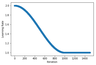 <!--notebook-skip-line-->
+ <!--notebook-skip-line-->
## Custom Schedule Modifiers
@@ -172,7 +172,7 @@ plot_schedule(schedule)
```
-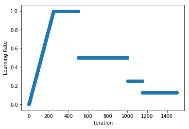 <!--notebook-skip-line-->
+ <!--notebook-skip-line-->
### Cool-Down
@@ -217,7 +217,7 @@ plot_schedule(schedule)
```
-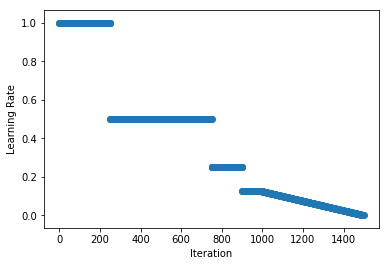 <!--notebook-skip-line-->
+ <!--notebook-skip-line-->
#### 1-Cycle: for "Super-Convergence"
@@ -257,7 +257,7 @@ plot_schedule(schedule)
```
-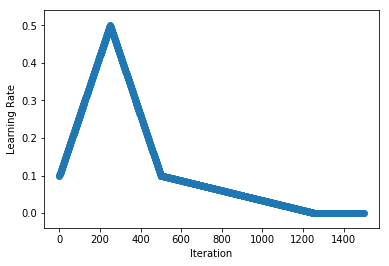 <!--notebook-skip-line-->
+ <!--notebook-skip-line-->
### Cyclical
@@ -304,7 +304,7 @@ plot_schedule(schedule)
```
-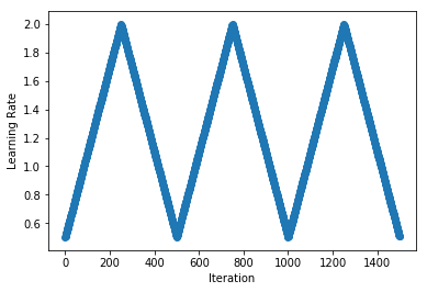 <!--notebook-skip-line-->
+ <!--notebook-skip-line-->
And lastly, we implement the scheduled used in ["SGDR: Stochastic Gradient Descent with Warm Restarts" by Ilya Loshchilov, Frank Hutter (2016)](https://arxiv.org/abs/1608.03983). We repeat cosine annealing schedules, but each time we halve the magnitude and double the cycle length.
@@ -317,7 +317,7 @@ plot_schedule(schedule)
```
-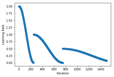 <!--notebook-skip-line-->
+ <!--notebook-skip-line-->
**_Want to learn more?_** Checkout the "Learning Rate Schedules" tutorial for a more basic overview of learning rates found in `mx.lr_scheduler`, and an example of how to use them while training your own models.
diff --git a/docs/python_docs/python/tutorials/packages/gluon/training/normalization/index.md b/docs/python_docs/python/tutorials/packages/gluon/training/normalization/index.md
index c17abe1..8c18b62 100644
--- a/docs/python_docs/python/tutorials/packages/gluon/training/normalization/index.md
+++ b/docs/python_docs/python/tutorials/packages/gluon/training/normalization/index.md
@@ -65,9 +65,9 @@ Advanced: all of the following methods begin by normalizing certain input distri
## Batch Normalization
-Figure 1: `BatchNorm` on NCHW data | Figure 2: `BatchNorm` on NTC data
-- | -
- | 
+Figure 1: `BatchNorm` on NCHW data | Figure 2: `BatchNorm` on NTC data
+- | -
+ | 
(e.g. batch of images) using the default of `axis=1` | (e.g. batch of sequences) overriding the default with `axis=2` (or `axis=-1`)
One of the most popular normalization techniques is Batch Normalization, usually called BatchNorm for short. We normalize the activations **across all samples in a batch** for each of the channels independently. See Figure 1. We calculate two batch (or local) statistics for every channel to perform the normalization: the mean and variance of the activations in that channel for all samples in a batch. And we use these to shift and scale respectively.
@@ -203,9 +203,9 @@ Warning: currently MXNet Gluon's implementation of `LayerNorm` is applied along
Remember: `LayerNorm` is intended to be used with data in NTC format so the default normalization axis is set to -1 (corresponding to C for channel). Change this to `axis=1` if you need to apply `LayerNorm` to data in NCHW format.
-Figure 3: `LayerNorm` on NCHW data | Figure 4: `LayerNorm` on NTC data
-- | -
- | 
+Figure 3: `LayerNorm` on NCHW data | Figure 4: `LayerNorm` on NTC data
+- | -
+ | 
(e.g. batch of images) overriding the default with `axis=1` | (e.g. batch of sequences) using the default of `axis=-1`
As an example, we'll apply `LayerNorm` to a batch of 2 samples, each with 4 time steps and 2 channels (in NTC format).
@@ -242,9 +242,9 @@ Another less common normalization technique is called `InstanceNorm`, which can
Watch out: `InstanceNorm` is better suited to convolutional networks (CNNs) than recurrent networks (RNNs). We expect the input distribution to the recurrent cell to change over time, so normalization over time doesn't work well. LayerNorm is better suited for this case.
-Figure 3: `InstanceNorm` on NCHW data | Figure 4: `InstanceNorm` on NTC data
-- | -
- | 
+Figure 3: `InstanceNorm` on NCHW data | Figure 4: `InstanceNorm` on NTC data
+- | -
+ | 
(e.g. batch of images) using the default `axis=1` | (e.g. batch of sequences) overiding the default with `axis=2` (or `axis=-1` equivalently)
As an example, we'll apply `InstanceNorm` to a batch of 2 samples, each with 2 channels, and both height and width of 2 (in NCHW format).
diff --git a/docs/python_docs/python/tutorials/packages/gluon/training/trainer.md b/docs/python_docs/python/tutorials/packages/gluon/training/trainer.md
index 8369a56..05be542 100644
--- a/docs/python_docs/python/tutorials/packages/gluon/training/trainer.md
+++ b/docs/python_docs/python/tutorials/packages/gluon/training/trainer.md
@@ -21,9 +21,9 @@ Training a neural network model consists of iteratively performing three simple
The first step is the forward step which computes the loss. In MXNet Gluon, this first step is achieved by doing a forward pass by calling `net.forward(X)` or simply `net(X)` and then calling the loss function with the result of the forward pass and the labels. For example `l = loss_fn(net(X), y)`.
-The second step is the backward step which computes the gradient of the loss with respect to the parameters. In Gluon, this step is achieved by doing the first step in an [autograd.record()](/api/python/docs/api/autograd/index.html) scope to record the computations needed to calculate the loss, and then calling `l.backward()` to compute the gradient of the loss with respect to the parameters.
+The second step is the backward step which computes the gradient of the loss with respect to the parameters. In Gluon, this step is achieved by doing the first step in an [autograd.record()](../../../../api/autograd/index.rst#mxnet.autograd.record) scope to record the computations needed to calculate the loss, and then calling `l.backward()` to compute the gradient of the loss with respect to the parameters.
-The final step is to update the neural network model parameters using an optimization algorithm. In Gluon, this step is performed by the [gluon.Trainer](/api/python/docs/api/gluon/trainer.html) and is the subject of this guide. When creating a Gluon `Trainer` you must provide a collection of parameters that need to be learnt. You also provide an `Optimizer` that will be used to update the parameters every training iteration when `trainer.step` is called.
+The final step is to update the neural network model parameters using an optimization algorithm. In Gluon, this step is performed by the [gluon.Trainer](../../../../api/gluon/trainer.rst#mxnet.gluon.Trainer) and is the subject of this guide. When creating a Gluon `Trainer` you must provide a collection of parameters that need to be learnt. You also provide an `Optimizer` that will be used to update the parameters every training iteration when `trainer.step` is called.
## Basic Usage
@@ -97,7 +97,7 @@ print(curr_weight - net.weight.grad() * 1 / batch_size)
In the previous example, we use the string argument `sgd` to select the optimization method, and `optimizer_params` to specify the optimization method arguments.
-All pre-defined optimization methods can be passed in this way and the complete list of implemented optimizers is provided in the [mxnet.optimizer](/api/python/docs/api/optimizer/index.html) module.
+All pre-defined optimization methods can be passed in this way and the complete list of implemented optimizers is provided in the [mxnet.optimizer](../../../../api/optimizer/index.rst) module.
However we can also pass an optimizer instance directly to the `Trainer` constructor.
@@ -114,14 +114,14 @@ trainer.step(batch_size)
net.weight.data()
```
-For reference and implementation details about each optimizer, please refer to the [guide](/api/python/docs/api/optimizer/index.html) for the `optimizer` module.
+For reference and implementation details about each optimizer, please refer to the [guide](../../optimizer/index.ipynb) and [API doc](../../../../api/optimizer/index.rst) for the `optimizer` module.
### KVStore Options
The `Trainer` constructor also accepts the following keyword arguments for :
-- `kvstore` – how key value store should be created for multi-gpu and distributed training. Check out [mxnet.kvstore.KVStore](/api/python/docs/api/kvstore/index.html) for more information. String options are any of the following ['local', 'device', 'dist_device_sync', 'dist_device_async'].
-- `compression_params` – Specifies type of gradient compression and additional arguments depending on the type of compression being used. See [mxnet.KVStore.set_gradient_compression_method](/api/python/docs/api/kvstore/index.html#mxnet.kvstore.KVStore.set_gradient_compression) for more details on gradient compression.
+- `kvstore` – how key value store should be created for multi-gpu and distributed training. Check out [mxnet.kvstore.KVStore](../../../../api/kvstore/index.rst) for more information. String options are any of the following ['local', 'device', 'dist_device_sync', 'dist_device_async'].
+- `compression_params` – Specifies type of gradient compression and additional arguments depending on the type of compression being used. See [mxnet.KVStore.set_gradient_compression_method](../../../../api/kvstore/generated/mxnet.kvstore.KVStore.rst) for more details on gradient compression.
- `update_on_kvstore` – Whether to perform parameter updates on KVStore. If None, then the `Trainer` instance will choose the more suitable option depending on the type of KVStore.
### Changing the Learning Rate
@@ -143,7 +143,7 @@ trainer.learning_rate
-In addition, there are multiple pre-defined learning rate scheduling methods that are already implemented in the [mxnet.lr_scheduler](/api/python/docs/api/lr_scheduler/index.html) module. The learning rate schedulers can be incorporated into your trainer by passing them in as an `optimizer_param` entry. Please refer to the [LR scheduler guide](/api/python/docs/tutorials/packages/gluon/training/learning_rates/learning_rate_schedules.html) to learn more.
+In addition, there are multiple pre-defined learning rate scheduling methods that are already implemented in the [mxnet.lr_scheduler](../../../../api/lr_scheduler/index.rst) module. The learning rate schedulers can be incorporated into your trainer by passing them in as an `optimizer_param` entry. Please refer to the [LR scheduler guide](./learning_rates/learning_rate_schedules.ipynb) to learn more.
@@ -160,9 +160,9 @@ In addition, there are multiple pre-defined learning rate scheduling methods tha
While optimization and optimizers play a significant role in deep learning model training, there are still other important components to model training. Here are a few suggestions about where to look next.
-* The [Optimizer API](/api/python/docs/api/optimizer/index.html) and [optimizer guide](/api/python/docs/tutorials/packages/optimizer/index.html) have information about all the different optimizers implemented in MXNet and their update steps. The [Dive into Deep Learning](https://en.diveintodeeplearning.org/chapter_optimization/index.html) book also has a chapter dedicated to optimization methods and explains various key optimizers in great detail.
+* The [Optimizer API](../../../../api/optimizer/index.rst) and [optimizer guide](../../optimizer/index.ipynb) have information about all the different optimizers implemented in MXNet and their update steps. The [Dive into Deep Learning](http://d2l.ai/chapter_optimization/index.html) book also has a chapter dedicated to optimization methods and explains various key optimizers in great detail.
-- Take a look at the [guide to parameter initialization](/api/python/docs/tutorials/packages/gluon/blocks/init.html) in MXNet to learn about what initialization schemes are already implemented, and how to implement your custom initialization schemes.
-- Also check out this [guide on parameter management](/api/python/docs/tutorials/packages/gluon/blocks/parameters.html) to learn about how to manage model parameters in gluon.
-- Make sure to take a look at the [guide to scheduling learning rates](/api/python/docs/tutorials/packages/gluon/training/learning_rates/learning_rate_schedules.html) to learn how to create learning rate schedules to make your training converge faster.
-- Finally take a look at the [KVStore API](/api/python/docs/api/kvstore/index.html) to learn how parameter values are synchronized over multiple devices.
+- Take a look at the [guide to parameter initialization](../blocks/init.ipynb) in MXNet to learn about what initialization schemes are already implemented, and how to implement your custom initialization schemes.
+- Also check out this [guide on parameter management](../blocks/parameters.ipynb) to learn about how to manage model parameters in gluon.
+- Make sure to take a look at the [guide to scheduling learning rates](./learning_rates/learning_rate_schedules.ipynb) to learn how to create learning rate schedules to make your training converge faster.
+- Finally take a look at the [KVStore API](../../../../api/kvstore/index.rst) to learn how parameter values are synchronized over multiple devices.
diff --git a/docs/python_docs/python/tutorials/packages/kvstore/kvstore.md b/docs/python_docs/python/tutorials/packages/kvstore/kvstore.md
index 8150290..e7b97c0 100644
--- a/docs/python_docs/python/tutorials/packages/kvstore/kvstore.md
+++ b/docs/python_docs/python/tutorials/packages/kvstore/kvstore.md
@@ -166,6 +166,6 @@ When the distributed version is ready, we will update this section.
<!-- flexibly as your choice. -->
## Next Steps
-* [MXNet tutorials index](/api/python/docs/tutorials/)
+* [MXNet tutorials index](../../index.rst)
<!-- INSERT SOURCE DOWNLOAD BUTTONS -->
diff --git a/docs/python_docs/python/tutorials/packages/legacy/ndarray/01-ndarray-intro.md b/docs/python_docs/python/tutorials/packages/legacy/ndarray/01-ndarray-intro.md
index 750f66a..6daba7a 100644
--- a/docs/python_docs/python/tutorials/packages/legacy/ndarray/01-ndarray-intro.md
+++ b/docs/python_docs/python/tutorials/packages/legacy/ndarray/01-ndarray-intro.md
@@ -26,7 +26,7 @@ This content was extracted and simplified from the gluon tutorials in
[Dive Into Deep Learning](https://d2l.ai/).
## Prerequisites
-* [MXNet installed in a Python environment](/get_started?version=master&platform=linux&language=python&environ=pip&processor=cpu).
+* [MXNet installed in a Python environment](https://mxnet.apache.org/get_started?version=master&platform=linux&language=python&environ=pip&processor=cpu).
* Python 2.7.x or Python 3.x
@@ -91,7 +91,7 @@ print(x)
```
Similarly, `ndarray` has a function to create a matrix of all ones aptly named
-[ones](/api/python/docs/api/ndarray/ndarray.html#mxnet.ndarray.ones).
+[ones](../../../../api/legacy/ndarray/ndarray.rst#mxnet.ndarray.ones).
```{.python .input}
x = nd.ones((3, 4))
@@ -102,7 +102,7 @@ Often, we'll want to create arrays whose values are sampled randomly. This is
especially common when we intend to use the array as a parameter in a neural
network. In this snippet, we initialize with values drawn from a standard normal
distribution with zero mean and unit variance using
-[random_normal](/api/python/docs/api/ndarray/ndarray.html#mxnet.ndarray.random_normal).
+[random_normal](../../../../api/legacy/ndarray/ndarray.rst#mxnet.ndarray.random_normal).
<!--
Is it that important to introduce zero mean and unit variance right now?
diff --git a/docs/python_docs/python/tutorials/packages/legacy/ndarray/02-ndarray-operations.md b/docs/python_docs/python/tutorials/packages/legacy/ndarray/02-ndarray-operations.md
index c2270f7..fd5213d 100644
--- a/docs/python_docs/python/tutorials/packages/legacy/ndarray/02-ndarray-operations.md
+++ b/docs/python_docs/python/tutorials/packages/legacy/ndarray/02-ndarray-operations.md
@@ -24,7 +24,7 @@ This content was extracted and simplified from the gluon tutorials in
[Dive Into Deep Learning](https://d2l.ai/).
## Prerequisites
-* [MXNet installed in a Python environment](/get_started).
+* [MXNet installed in a Python environment](https://mxnet.apache.org/get_started).
* Python 2.7.x or Python 3.x
diff --git a/docs/python_docs/python/tutorials/packages/legacy/ndarray/03-ndarray-contexts.md b/docs/python_docs/python/tutorials/packages/legacy/ndarray/03-ndarray-contexts.md
index 006d77c..ac3687f 100644
--- a/docs/python_docs/python/tutorials/packages/legacy/ndarray/03-ndarray-contexts.md
+++ b/docs/python_docs/python/tutorials/packages/legacy/ndarray/03-ndarray-contexts.md
@@ -24,7 +24,7 @@ This content was extracted and simplified from the gluon tutorials in
[Dive Into Deep Learning](https://d2l.ai/).
## Prerequisites
-* [MXNet installed (with GPU support) in a Python environment](/get_started).
+* [MXNet installed (with GPU support) in a Python environment](https://mxnet.apache.org/get_started).
* Python 2.7.x or Python 3.x
* **One or more GPUs**
@@ -86,4 +86,4 @@ print(z)
## Next Up
-[Back to NDArray API Guides](.)
+[Back to NDArray API Guides](../../../../api/legacy/ndarray/index.rst)
diff --git a/docs/python_docs/python/tutorials/packages/legacy/ndarray/gotchas_numpy_in_mxnet.md b/docs/python_docs/python/tutorials/packages/legacy/ndarray/gotchas_numpy_in_mxnet.md
index 2518f52..8f4f153 100644
--- a/docs/python_docs/python/tutorials/packages/legacy/ndarray/gotchas_numpy_in_mxnet.md
+++ b/docs/python_docs/python/tutorials/packages/legacy/ndarray/gotchas_numpy_in_mxnet.md
@@ -24,29 +24,29 @@ Warning: The latest MXNet offers NumPy-compatible array class `mx.np.ndarray` an
## Asynchronous and non-blocking nature of Apache MXNet
-Instead of using NumPy arrays Apache MXNet offers its own array implementation named [NDArray](/api/python/docs/api/ndarray/index.html). `NDArray API` was intentionally designed to be similar to `NumPy`, but there are differences.
+Instead of using NumPy arrays Apache MXNet offers its own array implementation named [NDArray](../../../../api/legacy/ndarray/ndarray.rst). `NDArray API` was intentionally designed to be similar to `NumPy`, but there are differences.
-One key difference is in the way calculations are executed. Every `NDArray` manipulation in Apache MXNet is done in asynchronous, non-blocking way. That means, that when we write code like `c = a * b`, where both `a` and `b` are `NDArrays`, the function is pushed to the [Execution Engine](/api/architecture/overview.html#execution-engine), which starts the calculation. The function immediately returns back, and the user thread can continue execution, despite the fact that the calculation [...]
+One key difference is in the way calculations are executed. Every `NDArray` manipulation in Apache MXNet is done in asynchronous, non-blocking way. That means, that when we write code like `c = a * b`, where both `a` and `b` are `NDArrays`, the function is pushed to the [Execution Engine](https://mxnet.apache.org/api/architecture/overview.html#execution-engine), which starts the calculation. The function immediately returns back, and the user thread can continue execution, despite the f [...]
`Execution Engine` builds the computation graph which may reorder or combine some calculations, but it honors dependency order: if there are other manipulation with `c` done later in the code, the `Execution Engine` will start doing them once the result of `c` is available. We don't need to write callbacks to start execution of subsequent code - the `Execution Engine` is going to do it for us.
To get the result of the computation we only need to access the resulting variable, and the flow of the code will be blocked until the computation results are assigned to the resulting variable. This behavior allows to increase code performance while still supporting imperative programming mode.
-Refer to the [intro tutorial to NDArray](/api/python/docs/tutorials/packages/ndarray/index.html), if you are new to Apache MXNet and would like to learn more how to manipulate NDArrays.
+Refer to the [intro tutorial to NDArray](./index.ipynb), if you are new to Apache MXNet and would like to learn more how to manipulate NDArrays.
## Converting NDArray to NumPy Array blocks calculation
-Many people are familiar with NumPy and flexible doing tensor manipulations using it. `NDArray API` offers a convinient [.asnumpy() method](/api/python/docs/api/ndarray/ndarray.html#mxnet.ndarray.NDArray.asnumpy) to cast `nd.array` to `np.array`. However, by doing this cast and using `np.array` for calculation, we cannot use all the goodness of `Execution Engine`. All manipulations done on `np.array` are blocking. Moreover, the cast to `np.array` itself is a blocking operation (same as [...]
+Many people are familiar with NumPy and flexible doing tensor manipulations using it. `NDArray API` offers a convinient [.asnumpy() method](../../../../api/legacy/ndarray/ndarray.rst#mxnet.ndarray.NDArray.asnumpy) to cast `nd.array` to `np.array`. However, by doing this cast and using `np.array` for calculation, we cannot use all the goodness of `Execution Engine`. All manipulations done on `np.array` are blocking. Moreover, the cast to `np.array` itself is a blocking operation (same as [...]
That means that if we have a long computation graph and, at some point, we want to cast the result to `np.array`, it may feel like the casting takes a lot of time. But what really takes this time is `Execution Engine`, which finishes all the async calculations we have pushed into it to get the final result, which then will be converted to `np.array`.
-Because of the blocking nature of [.asnumpy() method](/api/python/docs/api/ndarray/ndarray.html#mxnet.ndarray.NDArray.asnumpy), using it reduces the execution performance, especially if the calculations are done on GPU: Apache MXNet has to copy data from GPU to CPU to return `np.array`.
+Because of the blocking nature of [.asnumpy() method](../../../../api/legacy/ndarray/ndarray.rst#mxnet.ndarray.NDArray.asnumpy), using it reduces the execution performance, especially if the calculations are done on GPU: Apache MXNet has to copy data from GPU to CPU to return `np.array`.
-The best solution is to **make manipulations directly on NDArrays by methods provided in [NDArray API](https://mxnet.apache.org/api/python/ndarray/ndarray.html)**.
+The best solution is to **make manipulations directly on NDArrays by methods provided in [NDArray API](../../../../api/legacy/ndarray/ndarray.rst)**.
## NumPy operators vs. NDArray operators
-Despite the fact that [NDArray API](/api/python/docs/api/ndarray/index.html) was specifically designed to be similar to `NumPy`, sometimes it is not easy to replace existing `NumPy` computations. The main reason is that not all operators, that are available in `NumPy`, are available in `NDArray API`. The list of currently available operators is available on [NDArray class page](/api/python/docs/api/ndarray/ndarray.html).
+Despite the fact that [NDArray API](../../../../api/legacy/ndarray/ndarray.rst) was specifically designed to be similar to `NumPy`, sometimes it is not easy to replace existing `NumPy` computations. The main reason is that not all operators, that are available in `NumPy`, are available in `NDArray API`. The list of currently available operators is available on [NDArray class page](../../../../api/legacy/ndarray/ndarray.rst).
If a required operator is missing from `NDArray API`, there are few things you can do.
@@ -75,9 +75,9 @@ np.array_equal(np_y, nd_y.asnumpy())
### Find similar operator with different name and/or signature
-Some operators may have slightly different name, but are similar in terms of functionality. For example [nd.ravel_multi_index()](/api/python/docs/api/ndarray/ndarray.html#mxnet.ndarray.ravel_multi_index) is similar to [np.ravel()](https://docs.scipy.org/doc/numpy-1.14.0/reference/generated/numpy.ma.ravel.html#numpy.ma.ravel). In other cases some operators may have similar names, but different signatures. For example [np.split()](https://docs.scipy.org/doc/numpy-1.14.0/reference/generated [...]
+Some operators may have slightly different name, but are similar in terms of functionality. For example [nd.ravel_multi_index()](../../../../api/legacy/ndarray/ndarray.rst#mxnet.ndarray.ravel_multi_index) is similar to [np.ravel()](https://docs.scipy.org/doc/numpy-1.14.0/reference/generated/numpy.ma.ravel.html#numpy.ma.ravel). In other cases some operators may have similar names, but different signatures. For example [np.split()](https://docs.scipy.org/doc/numpy-1.14.0/reference/generate [...]
-One particular example of different input requirements is [nd.pad()](/api/python/docs/api/ndarray/ndarray.html#mxnet.ndarray.pad). The trick is that it can only work with 4-dimensional tensors. If your input has less dimensions, then you need to expand its number before using `nd.pad()` as it is shown in the code block below:
+One particular example of different input requirements is [nd.pad()](../../../../api/legacy/ndarray/ndarray.rst#mxnet.ndarray.pad). The trick is that it can only work with 4-dimensional tensors. If your input has less dimensions, then you need to expand its number before using `nd.pad()` as it is shown in the code block below:
```{.python .input}
@@ -106,7 +106,7 @@ pad_array(nd.array([1, 2, 3]), max_length=10)
### Search for an operator on [Github](https://github.com/apache/incubator-mxnet/labels/Operator)
-Apache MXNet community is responsive to requests, and everyone is welcomed to contribute new operators. Have in mind, that there is always a lag between new operators being merged into the codebase and release of a next stable version. For example, [nd.diag()](https://github.com/apache/incubator-mxnet/pull/11643) operator was recently introduced to Apache MXNet, but on the moment of writing this tutorial, it is not in any stable release. You can always get all latest implementations by i [...]
+Apache MXNet community is responsive to requests, and everyone is welcomed to contribute new operators. Have in mind, that there is always a lag between new operators being merged into the codebase and release of a next stable version. For example, [nd.diag()](https://github.com/apache/incubator-mxnet/pull/11643) operator was recently introduced to Apache MXNet, but on the moment of writing this tutorial, it is not in any stable release. You can always get all latest implementations by i [...]
## How to minimize the impact of blocking calls
diff --git a/docs/python_docs/python/tutorials/packages/legacy/ndarray/sparse/csr.md b/docs/python_docs/python/tutorials/packages/legacy/ndarray/sparse/csr.md
index b14bec6..3a8bae3 100644
--- a/docs/python_docs/python/tutorials/packages/legacy/ndarray/sparse/csr.md
+++ b/docs/python_docs/python/tutorials/packages/legacy/ndarray/sparse/csr.md
@@ -30,7 +30,7 @@ For matrices of high sparsity (e.g. ~1% non-zeros = ~1% density), there are two
- memory consumption is reduced significantly
- certain operations are much faster (e.g. matrix-vector multiplication)
-You may be familiar with the CSR storage format in [SciPy](https://www.scipy.org/) and will note the similarities in MXNet's implementation. However there are some additional competitive features in `CSRNDArray` inherited from `NDArray`, such as non-blocking asynchronous evaluation and automatic parallelization that are not available in SciPy's flavor of CSR. You can find further explanations for evaluation and parallelization strategy in MXNet in the [NDArray tutorial](https://mxnet.apa [...]
+You may be familiar with the CSR storage format in [SciPy](https://www.scipy.org/) and will note the similarities in MXNet's implementation. However there are some additional competitive features in `CSRNDArray` inherited from `NDArray`, such as non-blocking asynchronous evaluation and automatic parallelization that are not available in SciPy's flavor of CSR. You can find further explanations for evaluation and parallelization strategy in MXNet in the [NDArray tutorial](../gotchas_numpy_ [...]
The introduction of `CSRNDArray` also brings a new attribute, `stype` as a holder for storage type info, to `NDArray`. You can query **ndarray.stype** now in addition to the oft-queried attributes such as **ndarray.shape**, **ndarray.dtype**, and **ndarray.context**. For a typical dense NDArray, the value of `stype` is **"default"**. For a `CSRNDArray`, the value of stype is **"csr"**.
@@ -38,12 +38,12 @@ The introduction of `CSRNDArray` also brings a new attribute, `stype` as a holde
To complete this tutorial, you will need:
-- MXNet. See the instructions for your operating system in [Setup and Installation](https://mxnet.io/get_started)
+- MXNet. See the instructions for your operating system in [Setup and Installation](https://mxnet.apache.org/get_started)
- [Jupyter](http://jupyter.org/)
```
pip install jupyter
```
-- Basic knowledge of NDArray in MXNet. See the detailed tutorial for NDArray in [NDArray - Imperative tensor operations on CPU/GPU](https://mxnet.apache.org/tutorials/basic/ndarray.html).
+- Basic knowledge of NDArray in MXNet. See the detailed tutorial for NDArray in [NDArray - Imperative tensor operations on CPU/GPU](../01-ndarray-intro.rst).
- SciPy - A section of this tutorial uses SciPy package in Python. If you don't have SciPy, the example in that section will be ignored.
- GPUs - A section of this tutorial uses GPUs. If you don't have GPUs on your machine, simply set the variable `gpu_device` (set in the GPUs section of this tutorial) to `mx.cpu()`.
@@ -400,7 +400,7 @@ Note that multi-dimensional indexing or slicing along a particular axis is curre
## Sparse Operators and Storage Type Inference
-Operators that have specialized implementation for sparse arrays can be accessed in `mx.nd.sparse`. You can read the [mxnet.ndarray.sparse API documentation](https://mxnet.apache.org/versions/master/api/python/ndarray/sparse.html) to find what sparse operators are available.
+Operators that have specialized implementation for sparse arrays can be accessed in `mx.nd.sparse`. You can read the [mxnet.ndarray.sparse API documentation](../../../../../api/legacy/ndarray/sparse/index.rst) to find what sparse operators are available.
```{.python .input}
@@ -489,7 +489,7 @@ dataiter = mx.io.NDArrayIter(data, labels, batch_size, last_batch_handle='discar
```
-You can also load data stored in the [libsvm file format](https://www.csie.ntu.edu.tw/~cjlin/libsvmtools/datasets/) using `mx.io.LibSVMIter`, where the format is: ``<label> <col_idx1>:<value1> <col_idx2>:<value2> ... <col_idxN>:<valueN>``. Each line in the file records the label and the column indices and data for non-zero entries. For example, for a matrix with 6 columns, ``1 2:1.5 4:-3.5`` means the label is ``1``, the data is ``[[0, 0, 1,5, 0, -3.5, 0]]``. More detailed examples of `m [...]
+You can also load data stored in the [libsvm file format](https://www.csie.ntu.edu.tw/~cjlin/libsvmtools/datasets/) using `mx.io.LibSVMIter`, where the format is: ``<label> <col_idx1>:<value1> <col_idx2>:<value2> ... <col_idxN>:<valueN>``. Each line in the file records the label and the column indices and data for non-zero entries. For example, for a matrix with 6 columns, ``1 2:1.5 4:-3.5`` means the label is ``1``, the data is ``[[0, 0, 1,5, 0, -3.5, 0]]``. More detailed examples of `m [...]
```{.python .input}
@@ -556,7 +556,7 @@ except mx.MXNetError as err:
## Next
-[Train a Linear Regression Model with Sparse Symbols](/api/python/docs/tutorials/packages/ndarray/sparse/train.html)
+[Train a Linear Regression Model with Gluon Sparse](./train_gluon.ipynb)
<!-- INSERT SOURCE DOWNLOAD BUTTONS -->
diff --git a/docs/python_docs/python/tutorials/packages/legacy/ndarray/sparse/row_sparse.md b/docs/python_docs/python/tutorials/packages/legacy/ndarray/sparse/row_sparse.md
index 8dcdc96..6003e4f 100644
--- a/docs/python_docs/python/tutorials/packages/legacy/ndarray/sparse/row_sparse.md
+++ b/docs/python_docs/python/tutorials/packages/legacy/ndarray/sparse/row_sparse.md
@@ -95,13 +95,13 @@ In this tutorial, we will describe what the row sparse format is and how to use
To complete this tutorial, we need:
-- MXNet. See the instructions for your operating system in [Setup and Installation](/get_started)
+- MXNet. See the instructions for your operating system in [Setup and Installation](https://mxnet.apache.org/get_started)
- [Jupyter](http://jupyter.org/)
```
pip install jupyter
```
-- Basic knowledge of NDArray in MXNet. See the detailed tutorial for NDArray in [NDArray - Imperative tensor operations on CPU/GPU](https://mxnet.apache.org/tutorials/basic/ndarray.html)
-- Understanding of [automatic differentiation with autograd](http://gluon.mxnet.io/chapter01_crashcourse/autograd.html)
+- Basic knowledge of NDArray in MXNet. See the detailed tutorial for NDArray in [NDArray - Imperative tensor operations on CPU/GPU](../01-ndarray-intro.rst)
+- Understanding of [automatic differentiation with autograd](../../../autograd/index.ipynb)
- GPUs - A section of this tutorial uses GPUs. If you don't have GPUs on your
machine, simply set the variable `gpu_device` (set in the GPUs section of this
tutorial) to `mx.cpu()`
@@ -554,8 +554,8 @@ sgd.update(0, weight, grad, momentum)
```
-Note that only [mxnet.optimizer.SGD](https://mxnet.apache.org/api/python/optimization/optimization.html#mxnet.optimizer.SGD), [mxnet.optimizer.Adam](https://mxnet.apache.org/api/python/optimization/optimization.html#mxnet.optimizer.Adam), and
-[mxnet.optimizer.AdaGrad](https://mxnet.apache.org/api/python/optimization/optimization.html#mxnet.optimizer.AdaGrad) support sparse updates in MXNet.
+Note that only [mxnet.optimizer.SGD](../../../../../api/optimizer/index.rst#mxnet.optimizer.SGD), [mxnet.optimizer.Adam](../../../../../api/optimizer/index.rst#mxnet.optimizer.Adam), and
+[mxnet.optimizer.AdaGrad](../../../../../api/optimizer/index.rst#mxnet.optimizer.AdaGrad) support sparse updates in MXNet.
## Advanced Topics
@@ -578,7 +578,7 @@ except mx.MXNetError as err:
## Next
-[Train a Linear Regression Model with Sparse Symbols](/api/python/docs/tutorials/packages/ndarray/sparse/train.html)
+[Train a Linear Regression Model with Gluon Sparse](./train_gluon.ipynb)
<!-- INSERT SOURCE DOWNLOAD BUTTONS -->
diff --git a/docs/python_docs/python/tutorials/packages/legacy/ndarray/sparse/train_gluon.md b/docs/python_docs/python/tutorials/packages/legacy/ndarray/sparse/train_gluon.md
index e150258..cf99b53 100644
--- a/docs/python_docs/python/tutorials/packages/legacy/ndarray/sparse/train_gluon.md
+++ b/docs/python_docs/python/tutorials/packages/legacy/ndarray/sparse/train_gluon.md
@@ -20,7 +20,7 @@
When working on machine learning problems, you may encounter situations where the input data is sparse (i.e. the majority of values are zero). One example of this is in recommendation systems. You could have millions of user and product features, but only a few of these features are present for each sample. Without special treatment, the sheer magnitude of the feature space can lead to out-of-memory situations and cause significant slowdowns when training and making predictions.
-MXNet supports a number of sparse storage types (often called `stype` for short) for these situations. In this tutorial, we'll start by generating some sparse data, write it to disk in the LibSVM format and then read back using the [LibSVMIter](/api/python/docs/api/mxnet/io/index.html#mxnet.io.LibSVMIter) for training. We use the Gluon API to train the model and leverage sparse storage types such as [CSRNDArray](/api/python/docs/api/ndarray/sparse/index.html#mxnet.ndarray.sparse.CSRNDArr [...]
+MXNet supports a number of sparse storage types (often called `stype` for short) for these situations. In this tutorial, we'll start by generating some sparse data, write it to disk in the LibSVM format and then read back using the [LibSVMIter](../../../../../api/legacy/io/index.rst#mxnet.io.LibSVMIter) for training. We use the Gluon API to train the model and leverage sparse storage types such as [CSRNDArray](../../../../../api/legacy/ndarray/sparse/index.rst#mxnet.ndarray.sparse.CSRNDA [...]
```{.python .input}
@@ -63,7 +63,7 @@ print('{:,.0f} non-zero elements'.format(data.data.size))
10,000 non-zero elements
```
-Our storage type is CSR (Compressed Sparse Row) which is the ideal type for sparse data along multiple axes. See [this in-depth tutorial](/api/python/docs/tutorials/packages/ndarray/sparse/csr.html) for more information. Just to confirm the generation process ran correctly, we can see that the vast majority of values are indeed zero. One of the first questions to ask would be how much memory is saved by storing this data in a [CSRNDArray](/api/python/docs/api/ndarray/sparse/index.html#mx [...]
+Our storage type is CSR (Compressed Sparse Row) which is the ideal type for sparse data along multiple axes. See [this in-depth tutorial](./csr.ipynb) for more information. Just to confirm the generation process ran correctly, we can see that the vast majority of values are indeed zero. One of the first questions to ask would be how much memory is saved by storing this data in a [CSRNDArray](../../../../../api/legacy/ndarray/sparse/index.rst#mxnet.ndarray.sparse.CSRNDArray) versus a stan [...]
```{.python .input}
@@ -94,9 +94,9 @@ Given the extremely high sparsity of the data, we observe a huge memory saving h
### Writing Sparse Data
-Since there is such a large size difference between dense and sparse storage formats here, we ideally want to store the data on disk in a sparse storage format too. MXNet supports a format called LibSVM and has a data iterator called [LibSVMIter](/api/python/docs/api/mxnet/io/index.html#mxnet.io.LibSVMIter) specifically for data formatted this way.
+Since there is such a large size difference between dense and sparse storage formats here, we ideally want to store the data on disk in a sparse storage format too. MXNet supports a format called LibSVM and has a data iterator called [LibSVMIter](../../../../../api/legacy/io/index.rst#mxnet.io.LibSVMIter) specifically for data formatted this way.
-A LibSVM file has a row for each sample, and each row starts with the label: in this case `0.0` or `1.0` since we have a classification task. After this we have a variable number of `key:value` pairs separated by spaces, where the key is column/feature index and the value is the value of that feature. When working with your own sparse data in a custom format you should try to convert your data into this format. We define a `save_as_libsvm` function to save the `data` ([CSRNDArray](/api/p [...]
+A LibSVM file has a row for each sample, and each row starts with the label: in this case `0.0` or `1.0` since we have a classification task. After this we have a variable number of `key:value` pairs separated by spaces, where the key is column/feature index and the value is the value of that feature. When working with your own sparse data in a custom format you should try to convert your data into this format. We define a `save_as_libsvm` function to save the `data` ([CSRNDArray](../../ [...]
```{.python .input}
@@ -148,9 +148,9 @@ Some storage overhead is introduced by serializing the data as characters (with
### Reading Sparse Data
-Using [LibSVMIter](/api/python/docs/api/mxnet/io/index.html#mxnet.io.LibSVMIter), we can quickly and easily load data into batches ready for training. Although Gluon [Dataset](/api/python/docs/api/gluon/data/index.html#mxnet.gluon.data.Dataset)s can be written to return sparse arrays, Gluon [DataLoader](/api/python/docs/api/gluon/data/index.html#mxnet.gluon.data.DataLoader)s currently convert each sample to dense before stacking up to create the batch. As a result, [LibSVMIter](/api/pyth [...]
+Using [LibSVMIter](../../../../../api/legacy/io/index.rst#mxnet.io.LibSVMIter), we can quickly and easily load data into batches ready for training. Although Gluon [Dataset](../../../../../api/gluon/data/index.rst#mxnet.gluon.data.Dataset)s can be written to return sparse arrays, Gluon [DataLoader](../../../../../api/gluon/data/index.rst#mxnet.gluon.data.DataLoader)s currently convert each sample to dense before stacking up to create the batch. As a result, [LibSVMIter](../../../../../ap [...]
-Similar to using a [DataLoader](/api/python/docs/api/gluon/data/index.html#mxnet.gluon.data.DataLoader), you must specify the required `batch_size`. Since we're dealing with sparse data and the column shape isn't explicitly stored in the LibSVM file, we additionally need to provide the shape of the data and label. Our [LibSVMIter](/api/python/docs/api/mxnet/io/index.html#mxnet.io.LibSVMIter) returns batches in a slightly different form to a [DataLoader](/api/python/docs/api/gluon/data/in [...]
+Similar to using a [DataLoader](../../../../../api/gluon/data/index.rst#mxnet.gluon.data.DataLoader), you must specify the required `batch_size`. Since we're dealing with sparse data and the column shape isn't explicitly stored in the LibSVM file, we additionally need to provide the shape of the data and label. Our [LibSVMIter](../../../../../api/legacy/io/index.rst#mxnet.io.LibSVMIter) returns batches in a slightly different form to a [DataLoader](../../../../../api/gluon/data/index.rst [...]
```{.python .input}
data_iter = mx.io.LibSVMIter(data_libsvm=filepath, data_shape=(num_features,), label_shape=(1,), batch_size=10)
@@ -214,7 +214,7 @@ Although results will change depending on system specifications and degree of sp
Our next step is to define a network. We have an input of 1,000,000 features and we want to make a binary prediction. We don't have any spatial or temporal relationships between features, so we'll use a 3 layer fully-connected network where the last layer has 1 output unit (with sigmoid activation). Since we're working with sparse data, we'd ideally like to use network operators that can exploit this sparsity for improved performance and memory efficiency.
-Gluon's [nn.Dense](/api/python/docs/api/gluon/nn/index.html#mxnet.gluon.nn.Dense) block can used with [CSRNDArray](/api/python/docs/api/ndarray/sparse/index.html#mxnet.ndarray.sparse.CSRNDArray) input arrays but it doesn't exploit the sparsity. Under the hood, [Dense](/api/python/docs/api/gluon/nn/index.html#mxnet.gluon.nn.Dense) uses the [FullyConnected](/api/python/docs/api/ndarray/ndarray.html#mxnet.ndarray.FullyConnected) operator which isn't optimized for [CSRNDArray](/api/python/do [...]
+Gluon's [nn.Dense](../../../../../api/gluon/nn/index.rst#mxnet.gluon.nn.Dense) block can used with [CSRNDArray](../../../../../api/legacy/ndarray/sparse/index.rst#mxnet.ndarray.sparse.CSRNDArray) input arrays but it doesn't exploit the sparsity. Under the hood, [Dense](../../../../../api/gluon/nn/index.rst#mxnet.gluon.nn.Dense) uses the [FullyConnected](../../../../../api/legacy/ndarray/ndarray.rst#mxnet.ndarray.FullyConnected) operator which isn't optimized for [CSRNDArray](../../../../ [...]
```{.python .input}
@@ -233,11 +233,11 @@ class FullyConnected(mx.gluon.HybridBlock):
return F.FullyConnected(x, weight, bias, num_hidden=self._units)
```
-Our `weight` and `bias` parameters are dense (see `stype='default'`) and so are their gradients (see `grad_stype='default'`). Our `weight` parameter has shape `(units, in_units)` because the [FullyConnected](/api/python/docs/api/ndarray/ndarray.html#mxnet.ndarray.FullyConnected) operator performs the following calculation:
+Our `weight` and `bias` parameters are dense (see `stype='default'`) and so are their gradients (see `grad_stype='default'`). Our `weight` parameter has shape `(units, in_units)` because the [FullyConnected](../../../../../api/legacy/ndarray/ndarray.rst#mxnet.ndarray.FullyConnected) operator performs the following calculation:
$$Y = XW^T + b$$
-We could instead have created our parameter with shape `(in_units, units)` and avoid the transpose of the weight matrix. We'll see why this is so important later on. And instead of [FullyConnected](/api/python/docs/api/ndarray/ndarray.html#mxnet.ndarray.FullyConnected) we could have used [mx.sparse.dot](/api/python/docs/api/ndarray/sparse/index.html?#mxnet.ndarray.sparse.dot) to fully exploit the sparsity of the [CSRNDArray](/api/python/docs/api/ndarray/sparse/index.html#mxnet.ndarray.sp [...]
+We could instead have created our parameter with shape `(in_units, units)` and avoid the transpose of the weight matrix. We'll see why this is so important later on. And instead of [FullyConnected](../../../../../api/legacy/ndarray/ndarray.rst#mxnet.ndarray.FullyConnected) we could have used [mx.sparse.dot](../../../../../api/legacy/ndarray/sparse/index.rst#mxnet.ndarray.sparse.dot) to fully exploit the sparsity of the [CSRNDArray](../../../../../api/legacy/ndarray/sparse/index.rst#mxnet [...]
```{.python .input}
@@ -258,7 +258,7 @@ class FullyConnectedSparse(mx.gluon.HybridBlock):
Once again, we're using a dense `weight`, so both `FullyConnected` and `FullyConnectedSparse` will return dense array outputs. When constructing a multi-layer network therefore, only the first layer needs to be optimized for sparse inputs. Our first layer is often responsible for reducing the feature dimension dramatically (e.g. 1,000,000 features down to 128 features). We'll set the number of units in our 3 layers to be 128, 8 and 1.
-We will use [timeit](https://docs.python.org/2/library/timeit.html) to check the performance of these two variants, and analyse some [MXNet Profiler](/api/python/docs/tutorials/performance/backend/profiler.html) traces that have been created from these benchmarks. Additionally, we will inspect the memory usage of the weights (and gradients) using the `print_memory_allocation` function defined below:
+We will use [timeit](https://docs.python.org/2/library/timeit.html) to check the performance of these two variants, and analyse some [MXNet Profiler](../../../../performance/backend/profiler.rst) traces that have been created from these benchmarks. Additionally, we will inspect the memory usage of the weights (and gradients) using the `print_memory_allocation` function defined below:
```{.python .input}
@@ -321,7 +321,7 @@ for batch in data_iter:
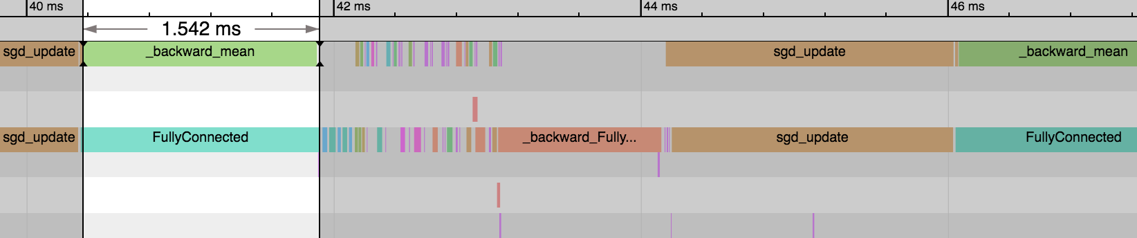
-We can see the first [FullyConnected](/api/python/docs/api/ndarray/ndarray.html#mxnet.ndarray.FullyConnected) operator takes a significant proportion of time to execute (~25% of the iteration) because there are 1,000,000 input features (to 128). After this, the other [FullyConnected](/api/python/docs/api/ndarray/ndarray.html#mxnet.ndarray.FullyConnected) operators are much faster because they have input features of 128 (to 8) and 8 (to 1). On the backward pass, we see the same pattern (b [...]
+We can see the first [FullyConnected](../../../../../api/legacy/ndarray/ndarray.rst#mxnet.ndarray.FullyConnected) operator takes a significant proportion of time to execute (~25% of the iteration) because there are 1,000,000 input features (to 128). After this, the other [FullyConnected](../../../../../api/legacy/ndarray/ndarray.rst#mxnet.ndarray.FullyConnected) operators are much faster because they have input features of 128 (to 8) and 8 (to 1). On the backward pass, we see the same pa [...]
```{.python .input}
@@ -330,13 +330,13 @@ print_memory_allocation(net, block_idxs=[0, 2, 4])
```
Memory Allocation for Weight:
-512.000 MBs ( 99.999%) for dense0
- 0.004 MBs ( 0.001%) for dense1
- 0.000 MBs ( 0.000%) for dense2
+512.000 MBs ( 99.999%) for dense0
+ 0.004 MBs ( 0.001%) for dense1
+ 0.000 MBs ( 0.000%) for dense2
Memory Allocation for Weight Gradient:
-512.000 MBs ( 99.999%) for dense0
- 0.004 MBs ( 0.001%) for dense1
- 0.000 MBs ( 0.000%) for dense2
+512.000 MBs ( 99.999%) for dense0
+ 0.004 MBs ( 0.001%) for dense1
+ 0.000 MBs ( 0.000%) for dense2
```
### Benchmark: `FullyConnectedSparse`
@@ -381,7 +381,7 @@ for batch in data_iter:
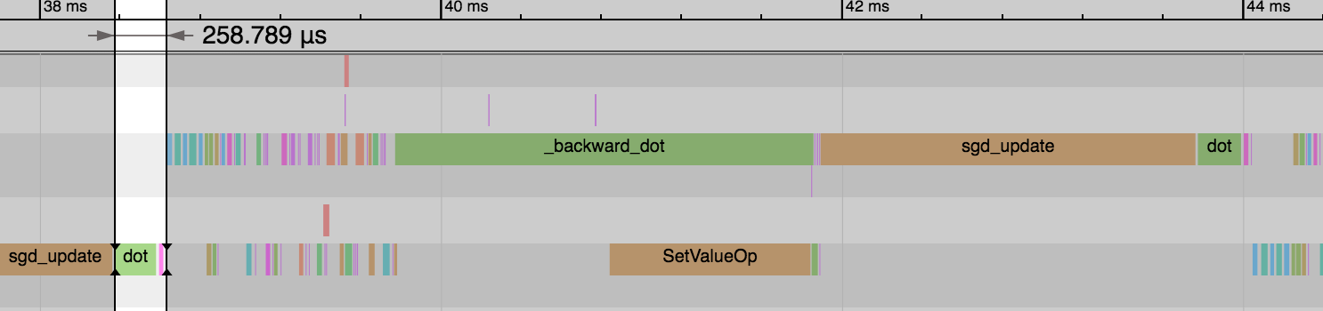
-We see the forward pass of `dot` and `add` (equivalent to [FullyConnected](/api/python/docs/api/ndarray/ndarray.html#mxnet.ndarray.FullyConnected) operator) is much faster now: 1.54ms vs 0.26ms. And this explains the reduction in overall time for the epoch. We didn't gain any benefit on the backward pass or parameter updates though.
+We see the forward pass of `dot` and `add` (equivalent to [FullyConnected](../../../../../api/legacy/ndarray/ndarray.rst#mxnet.ndarray.FullyConnected) operator) is much faster now: 1.54ms vs 0.26ms. And this explains the reduction in overall time for the epoch. We didn't gain any benefit on the backward pass or parameter updates though.
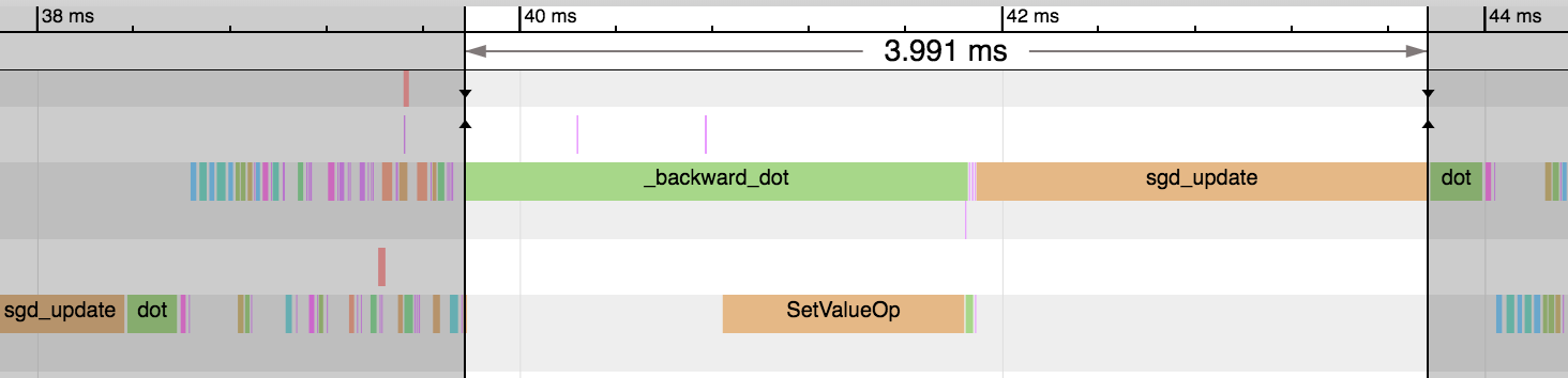
@@ -394,18 +394,18 @@ print_memory_allocation(net, block_idxs=[0, 2, 4])
```
Memory Allocation for Weight:
-512.000 MBs ( 99.999%) for fullyconnectedsparse0
- 0.004 MBs ( 0.001%) for fullyconnected0
- 0.000 MBs ( 0.000%) for fullyconnected1
+512.000 MBs ( 99.999%) for fullyconnectedsparse0
+ 0.004 MBs ( 0.001%) for fullyconnected0
+ 0.000 MBs ( 0.000%) for fullyconnected1
Memory Allocation for Weight Gradient:
-512.000 MBs ( 99.999%) for fullyconnectedsparse0
- 0.004 MBs ( 0.001%) for fullyconnected0
- 0.000 MBs ( 0.000%) for fullyconnected1
+512.000 MBs ( 99.999%) for fullyconnectedsparse0
+ 0.004 MBs ( 0.001%) for fullyconnected0
+ 0.000 MBs ( 0.000%) for fullyconnected1
```
-### Benchmark: `FullyConnectedSparse` with `grad_stype=row_sparse`
+### Benchmark: `FullyConnectedSparse` with `grad_stype=row_sparse`
-One useful outcome of sparsity in our [CSRNDArray](/api/python/docs/api/ndarray/sparse/index.html#mxnet.ndarray.sparse.CSRNDArray) input is that our gradients will be row sparse. We can exploit this fact to give us potentially huge memory savings and speed improvements. Creating our `weight` parameter with shape `(units, in_units)` and not transposing in the forward pass are important pre-requisite for obtaining row sparse gradients. Using [nn.Dense](/api/python/docs/api/gluon/nn/index.h [...]
+One useful outcome of sparsity in our [CSRNDArray](../../../../../api/legacy/ndarray/sparse/index.rst#mxnet.ndarray.sparse.CSRNDArray) input is that our gradients will be row sparse. We can exploit this fact to give us potentially huge memory savings and speed improvements. Creating our `weight` parameter with shape `(units, in_units)` and not transposing in the forward pass are important pre-requisite for obtaining row sparse gradients. Using [nn.Dense](../../../../../api/gluon/nn/index [...]
```{.python .input}
@@ -454,23 +454,21 @@ print_memory_allocation(net, block_idxs=[0, 2, 4])
```
Memory Allocation for Weight:
-512.000 MBs ( 99.999%) for fullyconnectedsparse1
- 0.004 MBs ( 0.001%) for fullyconnected2
- 0.000 MBs ( 0.000%) for fullyconnected3
+512.000 MBs ( 99.999%) for fullyconnectedsparse1
+ 0.004 MBs ( 0.001%) for fullyconnected2
+ 0.000 MBs ( 0.000%) for fullyconnected3
Memory Allocation for Weight Gradient:
- 0.059 MBs ( 93.490%) for fullyconnectedsparse1
- 0.004 MBs ( 6.460%) for fullyconnected2
- 0.000 MBs ( 0.050%) for fullyconnected3
+ 0.059 MBs ( 93.490%) for fullyconnectedsparse1
+ 0.004 MBs ( 6.460%) for fullyconnected2
+ 0.000 MBs ( 0.050%) for fullyconnected3
```
## Conclusion
-As part of this tutorial, we learned how to write sparse data to disk in LibSVM format and load it back in sparse batches with the [LibSVMIter](/api/python/docs/api/mxnet/io/index.html#mxnet.io.LibSVMIter). We learned how to improve the performance of Gluon's [nn.Dense](/api/python/docs/api/gluon/nn/index.html#mxnet.gluon.nn.Dense) on sparse arrays using `mx.nd.sparse`. And lastly, we set `grad_stype` to `'row_sparse'` to reduce the size of the gradient and speed up the parameter update step.
+As part of this tutorial, we learned how to write sparse data to disk in LibSVM format and load it back in sparse batches with the [LibSVMIter](../../../../../api/legacy/io/index.rst#mxnet.io.LibSVMIter). We learned how to improve the performance of Gluon's [nn.Dense](../../../../../api/gluon/nn/index.rst#mxnet.gluon.nn.Dense) on sparse arrays using `mx.nd.sparse`. And lastly, we set `grad_stype` to `'row_sparse'` to reduce the size of the gradient and speed up the parameter update step.
## Recommended Next Steps
-* More detail on the [CSRNDArray](/api/python/docs/api/ndarray/sparse/index.html#mxnet.ndarray.sparse.CSRNDArray) sparse array format can be found in [this tutorial](/api/python/docs/tutorials/packages/ndarray/sparse/csr.html).
-* More detail on the [RowSparseNDArray](/api/python/docs/api/ndarray/sparse/index.html#mxnet.ndarray.sparse.RowSparseNDArray) sparse array format can be found in [this tutorial](/api/python/docs/tutorials/packages/ndarray/sparse/row_sparse.html).
-* Users of the Module API can see a symbolic only example in [this tutorial](/api/python/docs/tutorials/packages/ndarray/sparse/train.html).
-
-<!-- INSERT SOURCE DOWNLOAD BUTTONS -->
+* More detail on the [CSRNDArray](../../../../../api/legacy/ndarray/sparse/index.rst#mxnet.ndarray.sparse.CSRNDArray) sparse array format can be found in [this tutorial](./csr.ipynb).
+* More detail on the [RowSparseNDArray](../../../../../api/legacy/ndarray/sparse/index.rst#mxnet.ndarray.sparse.RowSparseNDArray) sparse array format can be found in [this tutorial](./row_sparse.ipynb).
+* Users of the Gluon API can see a Gluon example in [this tutorial](./train_gluon.ipynb).
diff --git a/docs/python_docs/python/tutorials/packages/np/index.rst b/docs/python_docs/python/tutorials/packages/np/index.rst
index 3f1da88..6681676 100644
--- a/docs/python_docs/python/tutorials/packages/np/index.rst
+++ b/docs/python_docs/python/tutorials/packages/np/index.rst
@@ -16,7 +16,7 @@
under the License.
What is NP on MXNet
-=====================
+===================
NP on MXNet provides a NumPy-like interface with extensions
for deep learning. It contains two modules, ``mxnet.np``, which is similar to
@@ -29,4 +29,4 @@ If this is your first time using NP on MXNet, we recommend that you review the f
:maxdepth: 1
cheat-sheet
- np-vs-numpy
\ No newline at end of file
+ np-vs-numpy
diff --git a/docs/python_docs/python/tutorials/packages/np/np-vs-numpy.md b/docs/python_docs/python/tutorials/packages/np/np-vs-numpy.md
index 49be803..c406200 100644
--- a/docs/python_docs/python/tutorials/packages/np/np-vs-numpy.md
+++ b/docs/python_docs/python/tutorials/packages/np/np-vs-numpy.md
@@ -17,7 +17,7 @@
# Differences between NP on MXNet and NumPy
-This topic lists known differences between `mxnet.np` and `numpy`. With this quick reference, NumPy users can more easily adopt the MXNet NumPy-like API.
+This topic lists known differences between `mxnet.np` and `numpy`. With this quick reference, NumPy users can more easily adopt the MXNet NumPy-like API.
```{.python .input}
import numpy as onp # o means original
@@ -27,11 +27,11 @@ npx.set_np() # Configue MXNet to be NumPy-like
## Missing operators
-Many, but not all, operators in NumPy are supported in MXNet. You can find the missing operators in [NP on MXNet reference](/api/python/docs/api/ndarray/index.html). They're displayed in gray blocks instead of having links to their documents.
+Many, but not all, operators in NumPy are supported in MXNet. You can find the missing operators in [NP on MXNet reference](../../../api/np/index.rst). They're displayed in gray blocks instead of having links to their documents.
-In addition, an operator might not contain all arguments available in NumPy. For example, MXNet does not support stride. Check the operator document for more details.
+In addition, an operator might not contain all arguments available in NumPy. For example, MXNet does not support stride. Check the operator document for more details.
-## Extra functionalities
+## Extra functionalities
The `mxnet.np` module aims to mimic NumPy. Most extra functionalities that enhance NumPy for deep learning use are available on other modules, such as `npx` for operators used in deep learning and `autograd` for automatic differentiation. The `np` module API is not complete. One notable change is GPU support. Creating routines accepts a `ctx` argument:
@@ -42,7 +42,7 @@ b = np.random.uniform(ctx=gpu)
(a, b.context)
```
-Methods to move data across devices.
+Methods to move data across devices.
```{.python .input}
a.copyto(npx.cpu()), b.as_in_context(npx.cpu())
@@ -50,7 +50,7 @@ a.copyto(npx.cpu()), b.as_in_context(npx.cpu())
## Default data types
-NumPy uses 64-bit floating numbers or 64-bit integers by default.
+NumPy uses 64-bit floating numbers or 64-bit integers by default.
```{.python .input}
onp.array([1,2]).dtype, onp.array([1.2,2.3]).dtype
@@ -64,14 +64,14 @@ np.array([1,2]).dtype, np.array([1.2,2.3]).dtype
## Scalars
-NumPy has classes for scalars, whose base class is 'numpy.generic'. The return values of selecting an element and reduce operators are scalars.
+NumPy has classes for scalars, whose base class is 'numpy.generic'. The return values of selecting an element and reduce operators are scalars.
```{.python .input}
a = onp.array([1,2])
type(a[0]), type(a.sum())
```
-A scalar is almost identical to a 0-rank tensor (TODO, there may be subtle difference), but it has a different class. You can check the data type with `isinstance`
+A scalar is almost identical to a 0-rank tensor (TODO, there may be subtle difference), but it has a different class. You can check the data type with `isinstance`
```{.python .input}
b = a[0]
@@ -79,7 +79,7 @@ b = a[0]
isinstance(b, onp.int64), isinstance(b, onp.ndarray))
```
-MXNet returns 0-rank `ndarray` for scalars. (TODO, may consider to add scalar classes later.)
+MXNet returns 0-rank `ndarray` for scalars. (TODO, may consider to add scalar classes later.)
```{.python .input}
a = np.array([1,2])
diff --git a/docs/python_docs/python/tutorials/packages/onnx/fine_tuning_gluon.md b/docs/python_docs/python/tutorials/packages/onnx/fine_tuning_gluon.md
index 6e369fa..3080ad1 100644
--- a/docs/python_docs/python/tutorials/packages/onnx/fine_tuning_gluon.md
+++ b/docs/python_docs/python/tutorials/packages/onnx/fine_tuning_gluon.md
@@ -31,12 +31,12 @@ In this tutorial we will:
## Pre-requisite
To run the tutorial you will need to have installed the following python modules:
-- [MXNet > 1.1.0](/get_started)
+- [MXNet > 1.1.0](https://mxnet.apache.org/get_started)
- [onnx](https://github.com/onnx/onnx)
- matplotlib
We recommend that you have first followed this tutorial:
-- [Inference using an ONNX model on MXNet Gluon](/api/python/docs/tutorials/packages/onnx/inference_on_onnx_model.html)
+- [Inference using an ONNX model on MXNet Gluon](./inference_on_onnx_model.ipynb)
```{.python .input}
@@ -214,7 +214,7 @@ print(categories[dataset_train[N][1]])
-<!--notebook-skip-line-->
+<!--notebook-skip-line-->
## Fine-Tuning the ONNX model
@@ -449,7 +449,7 @@ plot_predictions(caltech101_images_test, result, categories, TOP_P)
```
-<!--notebook-skip-line-->
+<!--notebook-skip-line-->
**Great!** The network classified these images correctly after being fine-tuned on a dataset that contains images of `wrench`, `dolphin` and `lotus`
diff --git a/docs/python_docs/python/tutorials/packages/onnx/inference_on_onnx_model.md b/docs/python_docs/python/tutorials/packages/onnx/inference_on_onnx_model.md
index 518674b..c022f2a 100644
--- a/docs/python_docs/python/tutorials/packages/onnx/inference_on_onnx_model.md
+++ b/docs/python_docs/python/tutorials/packages/onnx/inference_on_onnx_model.md
@@ -21,7 +21,7 @@
[Open Neural Network Exchange (ONNX)](https://github.com/onnx/onnx) provides an open source format for AI models. It defines an extensible computation graph model, as well as definitions of built-in operators and standard data types.
In this tutorial we will:
-
+
- learn how to load a pre-trained .onnx model file into MXNet/Gluon
- learn how to test this model using the sample input/output
- learn how to test the model on custom images
@@ -29,7 +29,7 @@ In this tutorial we will:
## Pre-requisite
To run the tutorial you will need to have installed the following python modules:
-- [MXNet > 1.1.0](/get_started)
+- [MXNet > 1.1.0](https://mxnet.apache.org/get_started)
- [onnx](https://github.com/onnx/onnx) (follow the install guide)
- matplotlib
@@ -63,7 +63,7 @@ for image in images:
mx.test_utils.download(base_url.format(utils_file), fname=utils_file)
mx.test_utils.download(base_url.format(image_net_labels_file), fname=image_net_labels_file)
-from utils import *
+from utils import *
```
## Downloading a model from the ONNX model zoo
@@ -72,7 +72,7 @@ We download a pre-trained model, in our case the [GoogleNet](https://arxiv.org/a
```{.python .input}
-base_url = "https://s3.amazonaws.com/download.onnx/models/opset_3/"
+base_url = "https://s3.amazonaws.com/download.onnx/models/opset_3/"
current_model = "bvlc_googlenet"
model_folder = "model"
archive = "{}.tar.gz".format(current_model)
@@ -121,7 +121,7 @@ We pick a context, CPU is fine for inference, switch to mx.gpu() if you want to
ctx = mx.cpu()
```
-We obtain the data names of the inputs to the model by using the model metadata API:
+We obtain the data names of the inputs to the model by using the model metadata API:
```{.python .input}
model_metadata = onnx_mxnet.get_model_metadata(onnx_path)
@@ -138,10 +138,7 @@ data_names = [inputs[0] for inputs in model_metadata.get('input_tensor_data')]
print(data_names)
```
-
-```[u'data_0']```<!--notebook-skip-line-->
-
-And load them into a MXNet Gluon symbol block.
+And load them into a MXNet Gluon symbol block.
```{.python .input}
import warnings
@@ -173,7 +170,7 @@ mx.visualization.plot_network(sym, node_attrs={"shape":"oval","fixedsize":"fals
```
-<!--notebook-skip-line-->
+<!--notebook-skip-line-->
@@ -228,7 +225,7 @@ plot_predictions(image_net_images, result[:3], categories, TOP_P)
```
-<!--notebook-skip-line-->
+<!--notebook-skip-line-->
**Well done!** Looks like it is doing a pretty good job at classifying pictures when the category is a ImageNet label
@@ -252,5 +249,5 @@ We show that in our next tutorial:
- [Fine-tuning an ONNX Model using the modern imperative MXNet/Gluon](http://mxnet.apache.org/tutorials/onnx/fine_tuning_gluon.html)
-
+
<!-- INSERT SOURCE DOWNLOAD BUTTONS -->
diff --git a/docs/python_docs/python/tutorials/packages/optimizer/index.md b/docs/python_docs/python/tutorials/packages/optimizer/index.md
index d514e0e..bd19473 100644
--- a/docs/python_docs/python/tutorials/packages/optimizer/index.md
+++ b/docs/python_docs/python/tutorials/packages/optimizer/index.md
@@ -19,9 +19,9 @@
Deep learning models are comprised of a model architecture and the model parameters. The model architecture is chosen based on the task - for example Convolutional Neural Networks (CNNs) are very successful in handling image based tasks and Recurrent Neural Networks (RNNs) are better suited for sequential prediction tasks. However, the values of the model parameters are learned by solving an optimization problem during model training.
-To learn the parameters, we start with an initialization scheme and iteratively refine the parameter initial values by moving them along a direction that is opposite to the (approximate) gradient of the loss function. The extent to which the parameters are updated in this direction is governed by a hyperparameter called the learning rate. This process, known as gradient descent, is the backbone of optimization algorithms in deep learning. In MXNet, this functionality is abstracted by the [...]
+To learn the parameters, we start with an initialization scheme and iteratively refine the parameter initial values by moving them along a direction that is opposite to the (approximate) gradient of the loss function. The extent to which the parameters are updated in this direction is governed by a hyperparameter called the learning rate. This process, known as gradient descent, is the backbone of optimization algorithms in deep learning. In MXNet, this functionality is abstracted by the [...]
-When training a deep learning model using the MXNet [gluon API](/api/python/docs/tutorials/packages/gluon/index.html), a gluon [Trainer](/api/python/docs/tutorials/packages/gluon/training/trainer.html) is initialized with the all the learnable parameters and the optimizer to be used to learn those parameters. A single step of iterative refinement of model parameters in MXNet is achieved by calling [trainer.step](/api/python/docs/api/gluon/trainer.html#mxnet.gluon.Trainer.step) which in t [...]
+When training a deep learning model using the MXNet [Gluon API](../gluon/index.ipynb), a Gluon [Trainer](../gluon/training/trainer.ipynb) is initialized with the all the learnable parameters and the optimizer to be used to learn those parameters. A single step of iterative refinement of model parameters in MXNet is achieved by calling [Trainer.step](../../../api/gluon/trainer.rst#mxnet.gluon.Trainer.step) which in turn uses the gradient (and perhaps some state information) to update the [...]
Here is an example of how a trainer with an optimizer is created for, a simple Linear (Dense) Network.
@@ -35,7 +35,7 @@ optim = optimizer.SGD(learning_rate=0.1)
trainer = gluon.Trainer(net.collect_params(), optimizer=optim)
```
-In model training, the code snippet above would be followed by a training loop which, at every iteration performs a forward pass (to compute the loss), a backward pass (to compute the gradient of the loss with respect to the parameters) and a trainer step (which updates the parameters using the gradient). See the [gluon Trainer guide](/api/python/docs/tutorials/packages/gluon/training/trainer.html) for a complete example.
+In model training, the code snippet above would be followed by a training loop which, at every iteration performs a forward pass (to compute the loss), a backward pass (to compute the gradient of the loss with respect to the parameters) and a trainer step (which updates the parameters using the gradient). See the [Gluon Trainer guide](../gluon/training/trainer.ipynb) for a complete example.
We can also create the trainer by passing in the optimizer name and optimizer params into the trainer constructor directly, as shown below.
@@ -45,14 +45,14 @@ trainer = gluon.Trainer(net.collect_params(), optimizer='adam', optimizer_params
```
### What should I use?
-For many deep learning model architectures, the `sgd` and `adam` optimizers are a really good place to start. If you are implementing a deep learning model and trying to pick an optimizer, start with [sgd](/api/python/docs/api/optimizer/index.html#mxnet.optimizer.SGD) as you will often get good enough results as long as your learning problem is tractable. If you already have a trainable model and you want to improve the convergence then you can try [adam](/api/python/docs/api/optimizer/i [...]
+For many deep learning model architectures, the `sgd` and `adam` optimizers are a really good place to start. If you are implementing a deep learning model and trying to pick an optimizer, start with [SGD](../../../api/optimizer/index.rst#mxnet.optimizer.SGD) as you will often get good enough results as long as your learning problem is tractable. If you already have a trainable model and you want to improve the convergence then you can try [Adam](../../../api/optimizer/index.rst#mxnet.op [...]
## Stochastic Gradient Descent
-[Gradient descent](https://en.wikipedia.org/wiki/Gradient_descent) is a general purpose algorithm for minimizing a function using information from the gradient of the function with respect to its parameters. In deep learning, the function we are interested in minimizing is the [loss function](/api/python/docs/tutorials/packages/gluon/loss/loss.html). Our model accepts training data as inputs and the loss function tells us how good our model predictions are. Since the training data can ro [...]
+[Gradient descent](https://en.wikipedia.org/wiki/Gradient_descent) is a general purpose algorithm for minimizing a function using information from the gradient of the function with respect to its parameters. In deep learning, the function we are interested in minimizing is the [loss function](../gluon/loss/loss.ipynb). Our model accepts training data as inputs and the loss function tells us how good our model predictions are. Since the training data can routinely consist of millions of e [...]
Technically, stochastic gradient descent (SGD) refers to an online approximation of the gradient descent algorithm that computes the gradient of the loss function applied to a *single datapoint*, instead of your entire dataset, and uses this approximate gradient to update the model parameter values. However, in MXNet, and other deep learning frameworks, the SGD optimizer is agnostic to how many datapoints the loss function is applied to, and it is more effective to use a mini-batch loss [...]
-### [SGD optimizer](/api/python/docs/api/optimizer/index.html#mxnet.optimizer.SGD)
+### [SGD optimizer](../../../api/optimizer/index.rst#mxnet.optimizer.SGD)
For an SGD optimizer initialized with learning rate $lr$, the update function accepts parameters (weights) $w_i$, and their gradients $grad(w_i)$, and performs the single update step:
@@ -101,7 +101,7 @@ To create an SGD optimizer with momentum $\gamma$ and weight decay in MXNet simp
sgd_optimizer = optimizer.SGD(learning_rate=0.1, wd=0., momentum=0.8)
```
-### [Nesterov Accelerated Stochastic Gradient Descent](/api/python/docs/api/optimizer/index.html#mxnet.optimizer.NAG)
+### [Nesterov Accelerated Stochastic Gradient Descent](../../../api/optimizer/index.rst#mxnet.optimizer.NAG)
The momentum method of [Nesterov] is a modification to SGD with momentum that allows for even faster convergence in practice. With Nesterov accelerated gradient (NAG) descent, the update term is derived from the gradient of the loss function with respect to *refined parameter values*. These refined parameter values are computed by performing a SGD update step using the momentum history as the gradient term.
@@ -132,7 +132,7 @@ nag_optimizer = optimizer.NAG(learning_rate=0.1, momentum=0.8)
The gradient methods implemented by the optimizers described above use a global learning rate hyperparameter for all parameter updates. This has a well-documented shortcoming in that it makes the training process and convergence of the optimization algorithm really sensitive to the choice of the global learning rate. Adaptive learning rate methods avoid this pitfall by incorporating some history of the gradients observed in earlier iterations to scale step sizes (learning rates) to each [...]
-### [AdaGrad](/api/python/docs/api/optimizer/index.html#mxnet.optimizer.AdaGrad)
+### [AdaGrad](../../../api/optimizer/index.rst#mxnet.optimizer.AdaGrad)
The AdaGrad optimizer, which implements the optimization method originally described by [Duchi et al](http://www.jmlr.org/papers/volume12/duchi11a/duchi11a.pdf), multiplies the global learning rate by the $L_2$ norm of the preceeding gradient estimates for each paramater to obtain the per-parameter learning rate. To achieve this, AdaGrad introduces a new term which we'll denote as $g^2$ - the accumulated square of the gradient of the loss function with respect to the parameters.
@@ -152,7 +152,7 @@ To instantiate the Adagrad optimizer in MXNet you can use the following line of
adagrad_optimizer = optimizer.AdaGrad(learning_rate=0.1, eps=1e-07)
```
-### [RMSProp](/api/python/docs/api/optimizer/index.html#mxnet.optimizer.RMSProp)
+### [RMSProp](../../../api/optimizer/index.rst#mxnet.optimizer.RMSProp)
RMSProp, introduced by [Tielemen and Hinton](http://www.cs.toronto.edu/~tijmen/csc321/slides/lecture_slides_lec6.pdf), is similar to AdaGrad described above, but, instead of accumulating the sum of historical square gradients, maintains an exponential decaying average of the historical square gradients, in order to give more weighting to more recent gradients.
@@ -167,7 +167,7 @@ The $\epsilon$ term is included, as in AdaGrad, for numerical stability.
RMSProp was derived independently of AdaGrad and the name RMSProp derives from a combination of [RProp](https://en.wikipedia.org/wiki/Rprop) and the RMS, root mean square, operation in the denominator of the weight update.
-#### RMSProp (Centered)
+### RMSProp (Centered)
The MXNet RMSProp optimizer with the `centered=True` argument implements a variant of the RMSProp update described by [Alex Graves](https://arxiv.org/pdf/1308.0850v5.pdf), which centres the second moment $\mathbb{E}[g^2]$ or decaying average of square gradients by subtracting the square of decaying average of gradients. It also adds an explicit momentum term to weight past update steps. Representing the decaying average of gradients as $\mathbb{E}[g]$ and momentum parameter as $\gamma$, [...]
The centered RMSProp optimizer performs the update step:
@@ -186,7 +186,7 @@ rmsprop_optimizer = optimizer.RMSProp(learning_rate=0.001, rho=0.9, momentum=0.9
In the code snippet above, `rho` is $\beta$ in the equations above and `momentum` is $\gamma$, which is only used where `centered=True`.
-### [AdaDelta](/api/python/docs/api/optimizer/index.html#mxnet.optimizer.AdaDelta)
+### [AdaDelta](../../../api/optimizer/index.rst#mxnet.optimizer.AdaDelta)
AdaDelta was introduced to address some remaining lingering issues with AdaGrad and RMSProp - the selection of a global learning rate. AdaGrad and RMSProp assign each parameter its own learning rate but the per-parameter learning rate are still calculated using the global learning rate. In contrast, AdaDelta does not require a global learning rate, instead, it tracks the square of previous update steps, represented below as $\mathbb{E}[\Delta w^2]$ and uses the root mean square of the pr [...]
@@ -205,7 +205,7 @@ Here is the code snippet creating the AdaDelta optimizer in MXNet. The argument
adadelta_optimizer = optimizer.AdaDelta(rho=0.9, epsilon=1e-07)
```
-### [Adam](/api/python/docs/api/optimizer/index.html#mxnet.optimizer.Adam)
+### [Adam](../../../api/optimizer/index.rst#mxnet.optimizer.Adam)
Adam, introduced by [Kingma and Ba](https://arxiv.org/abs/1412.6980), is one of the popular adaptive algorithms for deep learning. It combines elements of RMSProp with momentum SGD. Like RMSProp, Adam uses the RootMeanSquare of decaying average of historical gradients but also explicitly keeps track of a decaying average of momentum and uses that for the update step direction. Thus, Adam accepts two hyperparameters $\beta_1$ and $\beta_2$ for momentum weighting and gradient RMS weighting [...]
The Adam optimizer performs the update step described the following equations:
@@ -223,7 +223,7 @@ In MXNet, you can construct the Adam optimizer with the following line of code.
adam_optimizer = optimizer.Adam(learning_rate=0.001, beta1=0.9, beta2=0.999, epsilon=1e-08)
```
-### [Adamax](/api/python/docs/api/optimizer/index.html#mxnet.optimizer.Adamax)
+### [Adamax](../../../api/optimizer/index.rst#mxnet.optimizer.Adamax)
Adamax is a variant of Adam also included in the original paper by [Kingma and Ba](https://arxiv.org/abs/1412.6980). Like Adam, Adamax maintains a moving average for first and second moments but Adamax uses the $L_{\infty}$ norm for the exponentially weighted average of the gradients, instead of the $L_2$ norm used in Adam used to keep track of the gradient second moment. The $L_{\infty}$ norm of a vector is equivalent to take the maximum absolute value of elements in that vector.
$$ v_{i+1} = \beta_1 \cdot v_{i} + (1 - \beta_1) \cdot grad(w_i) $$
@@ -238,7 +238,7 @@ See the code snippet below for how to construct Adamax in MXNet.
adamax_optimizer = optimizer.Adamax(learning_rate=0.002, beta1=0.9, beta2=0.999)
```
-### [Nadam](/api/python/docs/api/optimizer/index.html#mxnet.optimizer.Nadam)
+### [Nadam](../../../api/optimizer/index.rst#mxnet.optimizer.Nadam)
Nadam is also a variant of Adam and draws from the perspective that Adam can be viewed as a combination of RMSProp and classical Momentum (or Polyak Momentum). Nadam replaces the classical Momentum component of Adam with Nesterov Momentum (See [paper](http://cs229.stanford.edu/proj2015/054_report.pdf) by Dozat). The consequence of this is that the gradient used to update the weighted average of the momentum term is a lookahead gradient as is the case with NAG.
The Nadam optimizer performs the update step:
@@ -262,14 +262,15 @@ Training very deep neural networks can be time consuming and as such it is very
While all the preceding optimizers, from SGD to Adam, can be readily used in the distributed setting, the following optimizers in MXNet provide extra features targeted at alleviating some of the problems associated with distributed training.
-### [Signum](/api/python/docs/api/optimizer/index.html#mxnet.optimizer.Signum)
+### [Signum](../../../api/optimizer/index.rst#mxnet.optimizer.Signum)
In distributed training, communicating gradients across multiple worker nodes can be expensive and create a performance bottleneck. The Signum optimizer addresses this problem by transmitting just the sign of each minibatch gradient instead of the full precision gradient. In MXNet, the signum optimizer implements two variants of compressed gradients described in the paper by [Bernstein et al](https://arxiv.org/pdf/1802.04434.pdf).
The first variant, achieved by constructing the Signum optimizer with `momentum=0`, implements SignSGD update which performs the update below.
$$ w_{i+1} = w_i - lr \cdot sign(grad(w_i)) $$
-The second variant, achieved by passing a non-zero momentum parameter implements the Signum update which is equivalent to SignSGD and momentum. For momentum parameter $0 < \gamma < 1 $, the Signum optimizer performs the following update:
+The second variant, achieved by passing a non-zero momentum parameter implements the Signum update which is equivalent to SignSGD and momentum.
+For momentum parameter $\gamma \in [0, 1]$, the Signum optimizer performs the following update:
$$ v_{i+1} = \gamma \cdot v_i + (1 - \gamma) \cdot grad(w_i) $$
$$ w_{i+1} = w_i - lr \cdot sign(v_{i+1}) $$
@@ -282,7 +283,7 @@ signum_optimizer = optimizer.Signum(learning_rate=0.01, momentum=0.9, wd_lh=0.0)
```
-### [DCASGD](/api/python/docs/api/optimizer/index.html#mxnet.optimizer.DCASGD)
+### [DCASGD](../../../api/optimizer/index.rst#mxnet.optimizer.DCASGD)
The DCASGD optimizer implements Delay Compensated Asynchronous Stochastic Gradient Descent by [Zheng et al](https://arxiv.org/pdf/1609.08326.pdf). In asynchronous distributed SGD, it is possible that a training worker node add its gradients too late to the global (parameter) server resulting in a delayed gradient being used to update the current parameters. DCASGD addresses this issue of delayed gradients by compensating for this delay in the parameter update steps.
@@ -302,7 +303,7 @@ Before deep neural networks became popular post 2012, people were already solvin
The class of optimization algorithms designed to tackle online learning problems have also seen some success in offline training of deep neural models. The following optimizers are algorithms taken from online learning that have been implemented in MXNet.
-### [FTRL](/api/python/docs/api/optimizer/index.html#mxnet.optimizer.Ftrl)
+### [FTRL](../../../api/optimizer/index.rst#mxnet.optimizer.Ftrl)
FTRL stands for Follow the Regularized Leader and describes a family of algorithms originally designed for online learning tasks.
@@ -325,12 +326,14 @@ Here is how to initialize the FTRL optimizer in MXNet
ftrl_optimizer = optimizer.Ftrl(lamda1=0.01, learning_rate=0.1, beta=1)
```
-### [FTML](/api/python/docs/api/optimizer/index.html#mxnet.optimizer.FTML)
+### [FTML](../../../api/optimizer/index.rst#mxnet.optimizer.FTML)
FTML stands for Follow the Moving Leader and is a variant of the FTRL family of algorithms adapted specifically to deep learning. Regular FTRL algorithms, described above, solve an optimization problem every update that involves the sum of all previous gradients. This is not well suited for the non-convex loss functions in deep learning. In the non-convex settings, older gradients are likely uninformative as the parameter updates can move to converge towards different local minima at dif [...]
-$$ w_{i+1} = \texttt{argmin}_{w} \left[\sum_{j=1}^{i} (1 − \beta_1)\beta_1^{i−j} grad(w_i)\cdot w + \dfrac{1}{2}\sum_{j=1}^{i} \sigma_j \cdot ||w - w_j||_2^2 \right]$$
+\begin{equation*}
+w_{i+1} = \texttt{argmin}_{w} \left[\sum_{j=1}^{i} (1 − \beta_1)\beta_1^{i−j} grad(w_i)\cdot w + \dfrac{1}{2}\sum_{j=1}^{i} \sigma_j \cdot ||w - w_j||_2^2 \right]
+\end{equation*}
$\beta_1$ is introduced to compute the exponential moving average of the previous accumulated gradient. The improvements of FTML over FTRL can be compared to the improvements of RMSProp/Adam to AdaGrad. According to [Zheng et al](http://proceedings.mlr.press/v70/zheng17a/zheng17a.pdf), FTML enjoys some of the nice properties of RMSProp and Adam while avoiding their pitfalls.
@@ -353,7 +356,7 @@ Here `beta1` and `beta2` are similar to the arguments in the Adam optimizer.
## Bayesian SGD
A notable shortcoming of deep learning is that the model parameters learned after training are only point estimates, therefore deep learning model predictions have no information about uncertainty or confidence bounds. This is in contrast to a fully Bayesian approach which incorporates prior distributions on the model parameters and estimates the model parameters as belonging to a posterior distribution. This approach allows the predictions of a bayesian model to have information about u [...]
-### [SGLD](/api/python/docs/api/optimizer/index.html#mxnet.optimizer.SGLD)
+### [SGLD](../../../api/optimizer/index.rst#mxnet.optimizer.SGLD)
Stochastic Gradient Langevin Dynamics or SGLD was introduced to allow uncertainties around model parameters to be captured directly during model training. With every update in SGLD, the learning rate decreases to zero and a gaussian noise of known variances is injected into the SGD step. This has the effect of having the training parameters converge to a sufficient statistic for a posterior distribution instead of simply a point estimate of the model parameters.
SGLD performs the parameter update:
@@ -375,14 +378,14 @@ If you would like to use a particular optimizer that is not yet implemented in M
Step 1: First create a function that is able to perform your desired updates given the weights, gradients and other state information.
-Step 2: You will have to write your own optimizer class that extends the [base optimizer class](/api/python/docs/api/optimizer/index.html#mxnet.optimizer.Optimizer) and override the following functions
+Step 2: You will have to write your own optimizer class that extends the [base optimizer class](../../../api/optimizer/index.rst#mxnet.optimizer.Optimizer) and override the following functions
* `__init__`: accepts the parameters of your optimizer algorithm as inputs as saves them as member variables.
* `create_state`: If your custom optimizer uses some additional state information besides the gradient, then you should implement a function that accepts the weights and returns the state.
* `update`: Implement your optimizer update function using the function in Step 1
Step 3: Register your optimizer with `@register` decorator on your optimizer class.
-See the [source code](/api/python/docs/api/optimizer/index.html#mxnet.optimizer.NAG) for the NAG optimizer for a concrete example.
+See the [source code](../../../api/optimizer/index.rst#mxnet.optimizer.NAG) for the NAG optimizer for a concrete example.
## Summary
* MXNet implements many state-of-the-art optimizers which can be passed directly into a gluon trainer object. Calling `trainer.step` during model training uses the optimizers to update the model parameters.
@@ -395,9 +398,9 @@ See the [source code](/api/python/docs/api/optimizer/index.html#mxnet.optimizer.
## Next Steps
While optimization and optimizers play a significant role in deep learning model training, there are still other important components to model training. Here are a few suggestions about where to look next.
-* The [trainer API](/api/python/docs/api/gluon/trainer.html) and [guide](/api/python/docs/tutorials/packages/gluon/training/trainer.html) have information about how to construct the trainer that encapsulate the optimizers and will actually be used in your model training loop.
-* Check out the guide to MXNet gluon [Loss functions](/api/python/docs/tutorials/packages/gluon/loss/loss.html) and [custom losses](/api/python/docs/tutorials/packages/gluon/loss/custom-loss.html) to learn about the loss functions optimized by these optimizers, see what loss functions are already implemented in MXNet and understand how to write your own custom loss functions.
-* Take a look at the [guide to parameter initialization](/api/python/docs/tutorials/packages/gluon/blocks/init.html) in MXNet to learn about what initialization schemes are already implemented, and how to implement your custom initialization schemes.
-* Also check out the [autograd guide](/api/python/docs/tutorials/packages/autograd/index.html) to learn about automatic differentiation and how gradients are automatically computed in MXNet.
-* Make sure to take a look at the [guide to scheduling learning rates](/api/python/docs/tutorials/packages/gluon/training/learning_rates/learning_rate_schedules.html) to learn how to create learning rate schedules to supercharge the convergence of your optimizer.
-* Finally take a look at the [KVStore API](/api/python/docs/tutorials/packages/kvstore/index.html) to learn how parameter values are synchronized over multiple devices.
+* The [trainer API](../../../api/gluon/trainer.rst) and [guide](../gluon/training/trainer.ipynb) have information about how to construct the trainer that encapsulate the optimizers and will actually be used in your model training loop.
+* Check out the guide to MXNet gluon [Loss functions](../gluon/loss/loss.ipynb) and [custom losses](../gluon/loss/custom-loss.ipynb) to learn about the loss functions optimized by these optimizers, see what loss functions are already implemented in MXNet and understand how to write your own custom loss functions.
+* Take a look at the [guide to parameter initialization](../gluon/blocks/init.ipynb) in MXNet to learn about what initialization schemes are already implemented, and how to implement your custom initialization schemes.
+* Also check out the [autograd guide](../autograd/index.ipynb) to learn about automatic differentiation and how gradients are automatically computed in MXNet.
+* Make sure to take a look at the [guide to scheduling learning rates](../gluon/training/learning_rates/learning_rate_schedules.ipynb) to learn how to create learning rate schedules to supercharge the convergence of your optimizer.
+* Finally take a look at the [KVStore API](../kvstore/index.ipynb) to learn how parameter values are synchronized over multiple devices.
diff --git a/docs/python_docs/python/tutorials/performance/backend/profiler.md b/docs/python_docs/python/tutorials/performance/backend/profiler.md
index d34e5bb..ecd9fc8 100644
--- a/docs/python_docs/python/tutorials/performance/backend/profiler.md
+++ b/docs/python_docs/python/tutorials/performance/backend/profiler.md
@@ -235,7 +235,7 @@ Moreover, you can set `MKLDNN_VERBOSE=2` to collect both creating and executing
### Profiling Custom Operators
-Should the existing NDArray operators fail to meet all your model's needs, MXNet supports [Custom Operators](/api/python/docs/tutorials/extend/customop.html) that you can define in Python. In `forward()` and `backward()` of a custom operator, there are two kinds of code: "pure Python" code (NumPy operators included) and "sub-operators" (NDArray operators called within `forward()` and `backward()`). With that said, MXNet can profile the execution time of both kinds without additional setu [...]
+Should the existing NDArray operators fail to meet all your model's needs, MXNet supports [Custom Operators](../../extend/customop.ipynb) that you can define in Python. In `forward()` and `backward()` of a custom operator, there are two kinds of code: "pure Python" code (NumPy operators included) and "sub-operators" (NDArray operators called within `forward()` and `backward()`). With that said, MXNet can profile the execution time of both kinds without additional setup. Specifically, the [...]
Let's try profiling custom operators with the following code example:
@@ -316,7 +316,7 @@ profiler.dump()
MXNet's Profiler is the recommended starting point for profiling MXNet code, but NVIDIA also provides a couple of tools for low-level profiling of CUDA code: [NVProf](https://devblogs.nvidia.com/cuda-pro-tip-nvprof-your-handy-universal-gpu-profiler/), [Visual Profiler](https://developer.nvidia.com/nvidia-visual-profiler) and [Nsight Compute](https://developer.nvidia.com/nsight-compute). You can use these tools to profile all kinds of executables, so they can be used for profiling Python [...]
-#### NVProf and Visual Profiler
+### NVProf and Visual Profiler
NVProf and Visual Profiler are available in CUDA 9 and CUDA 10 toolkits. You can get a timeline view of CUDA kernel executions, and also analyse the profiling results to get automated recommendations. It is useful for profiling end-to-end training but the interface can sometimes become slow and unresponsive.
@@ -332,25 +332,25 @@ We specified an output file called `my_profile.nvvp` and this will be annotated
You can open this file in Visual Profiler to visualize the results.
-
+
At the top of the plot we have CPU tasks such as driver operations, memory copy calls, MXNet engine operator invocations, and imperative MXNet API calls. Below we see the kernels active on the GPU during the same time period.
-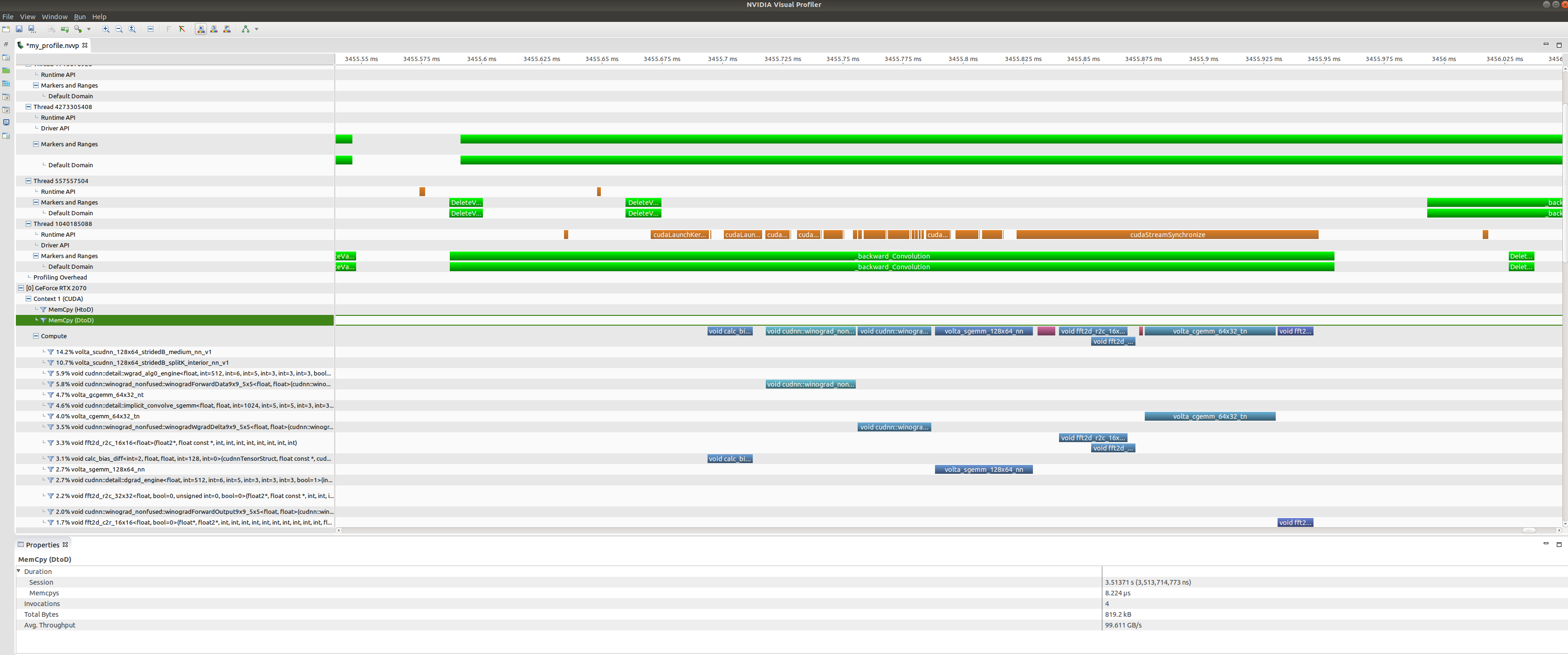
+
Zooming in on a backwards convolution operator we can see that it is in fact made up of a number of different GPU kernel calls, including a cuDNN winograd convolution call, and a fast-fourier transform call.
-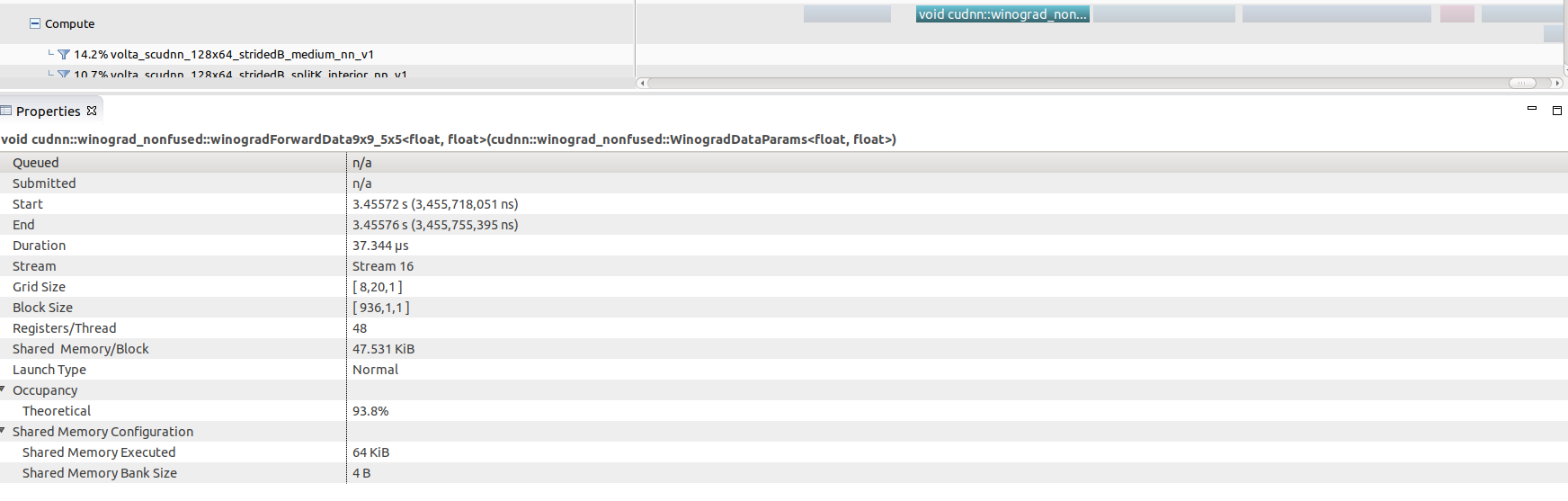
+
Selecting any of these kernel calls (the winograd convolution call shown here) will get you some interesting GPU performance information such as occupancy rates (vs theoretical), shared memory usage and execution duration.
-#### Nsight Compute
+### Nsight Compute
Nsight Compute is available in CUDA 10 toolkit, but can be used to profile code running CUDA 9. You don't get a timeline view, but you get many low level statistics about each individual kernel executed and can compare multiple runs (i.e. create a baseline).
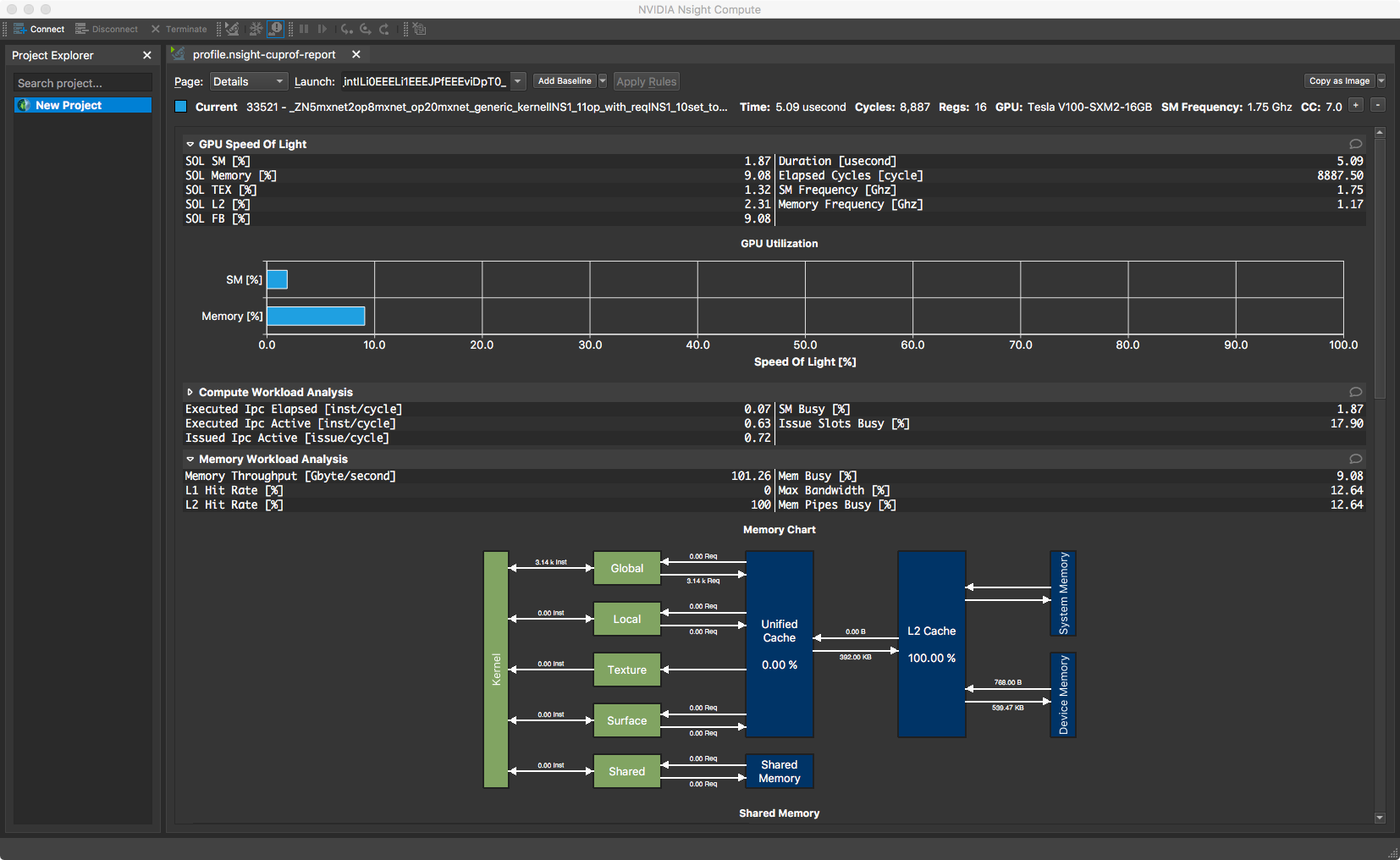
-### Further reading
+## Further reading
- [Examples using MXNet profiler.](https://github.com/apache/incubator-mxnet/tree/master/example/profiler)
- [Some tips for improving MXNet performance.](https://mxnet.apache.org/api/faq/perf)
diff --git a/python/mxnet/gluon/rnn/rnn_cell.py b/python/mxnet/gluon/rnn/rnn_cell.py
index 236354d..bb28533 100644
--- a/python/mxnet/gluon/rnn/rnn_cell.py
+++ b/python/mxnet/gluon/rnn/rnn_cell.py
@@ -1432,9 +1432,9 @@ def dynamic_unroll(cell, inputs, begin_state, drop_inputs=0, drop_outputs=0,
>>> state_shape = (batch_size, input_size)
>>> states = [mx.nd.normal(loc=0, scale=1, shape=state_shape) for i in range(2)]
>>> valid_length = mx.nd.array([2, 3])
- >>> output, states = mx.gluon.contrib.rnn.rnn_cell.dynamic_unroll(cell, rnn_data, states,
- valid_length=valid_length,
- layout='TNC')
+ >>> output, states = mx.gluon.rnn.rnn_cell.dynamic_unroll(cell, rnn_data, states,
+ ... valid_length=valid_length,
+ ... layout='TNC')
>>> print(output)
[[[ 0.00767238 0.00023103 0.03973929 -0.00925503 -0.05660512]
[ 0.00881535 0.05428379 -0.02493718 -0.01834097 0.02189514]]
diff --git a/python/mxnet/numpy/random.py b/python/mxnet/numpy/random.py
index ccfa433..3f10902 100644
--- a/python/mxnet/numpy/random.py
+++ b/python/mxnet/numpy/random.py
@@ -145,7 +145,6 @@ def normal(loc=0.0, scale=1.0, size=None, dtype=None, ctx=None, out=None):
Samples are distributed according to a normal distribution parametrized
by *loc* (mean) and *scale* (standard deviation).
-
Parameters
----------
loc : float, optional
@@ -169,7 +168,7 @@ def normal(loc=0.0, scale=1.0, size=None, dtype=None, ctx=None, out=None):
Returns
-------
out : ndarray
- Drawn samples from the parameterized normal distribution.
+ Drawn samples from the parameterized `normal distribution` [1]_.
Notes
-----
@@ -212,8 +211,8 @@ def normal(loc=0.0, scale=1.0, size=None, dtype=None, ctx=None, out=None):
def lognormal(mean=0.0, sigma=1.0, size=None, dtype=None, ctx=None, out=None):
r"""Draw samples from a log-normal distribution.
- Draw samples from a log-normal distribution with specified mean,
- standard deviation, and array shape. Note that the mean and standard
+ Draw samples from a `log-normal distribution` [1]_ with specified mean,
+ standard deviation, and array shape. Note that the mean and standard
deviation are not the values for the distribution itself, but of the
underlying normal distribution it is derived from.
@@ -244,10 +243,12 @@ def lognormal(mean=0.0, sigma=1.0, size=None, dtype=None, ctx=None, out=None):
Notes
-----
A variable `x` has a log-normal distribution if `log(x)` is normally
- distributed. The probability density function for the log-normal
- distribution is:
+ distributed. The `probability density function for the log-normal
+ distribution` [2]_ is:
+
.. math:: p(x) = \frac{1}{\sigma x \sqrt{2\pi}}
e^{(-\frac{(ln(x)-\mu)^2}{2\sigma^2})}
+
where :math:`\mu` is the mean and :math:`\sigma` is the standard
deviation of the normally distributed logarithm of the variable.
A log-normal distribution results if a random variable is the *product*
@@ -259,11 +260,11 @@ def lognormal(mean=0.0, sigma=1.0, size=None, dtype=None, ctx=None, out=None):
References
----------
.. [1] Limpert, E., Stahel, W. A., and Abbt, M., "Log-normal
- Distributions across the Sciences: Keys and Clues,"
- BioScience, Vol. 51, No. 5, May, 2001.
- https://stat.ethz.ch/~stahel/lognormal/bioscience.pdf
+ Distributions across the Sciences: Keys and Clues,"
+ BioScience, Vol. 51, No. 5, May, 2001.
+ https://stat.ethz.ch/~stahel/lognormal/bioscience.pdf
.. [2] Reiss, R.D. and Thomas, M., "Statistical Analysis of Extreme
- Values," Basel: Birkhauser Verlag, 2001, pp. 31-32.
+ Values," Basel: Birkhauser Verlag, 2001, pp. 31-32.
Examples
--------
@@ -276,8 +277,10 @@ def lognormal(mean=0.0, sigma=1.0, size=None, dtype=None, ctx=None, out=None):
def logistic(loc=0.0, scale=1.0, size=None, ctx=None, out=None):
r"""Draw samples from a logistic distribution.
+
Samples are drawn from a logistic distribution with specified
parameters, loc (location or mean, also median), and scale (>0).
+
Parameters
----------
loc : float or array_like of floats, optional
@@ -294,10 +297,12 @@ def logistic(loc=0.0, scale=1.0, size=None, ctx=None, out=None):
Device context of output, default is current context.
out : ``ndarray``, optional
Store output to an existing ``ndarray``.
+
Returns
-------
out : ndarray or scalar
Drawn samples from the parameterized logistic distribution.
+
Examples
--------
Draw samples from the distribution:
@@ -317,8 +322,10 @@ def logistic(loc=0.0, scale=1.0, size=None, ctx=None, out=None):
def gumbel(loc=0.0, scale=1.0, size=None, ctx=None, out=None):
r"""Draw samples from a Gumbel distribution.
+
Draw samples from a Gumbel distribution with specified location and
scale.
+
Parameters
----------
loc : float or array_like of floats, optional
@@ -335,10 +342,12 @@ def gumbel(loc=0.0, scale=1.0, size=None, ctx=None, out=None):
Device context of output, default is current context.
out : ``ndarray``, optional
Store output to an existing ``ndarray``.
+
Returns
-------
out : ndarray or scalar
Drawn samples from the parameterized Gumbel distribution.
+
Examples
--------
Draw samples from the distribution:
@@ -551,8 +560,10 @@ def choice(a, size=None, replace=True, p=None, ctx=None, out=None):
def rayleigh(scale=1.0, size=None, ctx=None, out=None):
r"""Draw samples from a Rayleigh distribution.
+
The :math:`\chi` and Weibull distributions are generalizations of the
Rayleigh.
+
Parameters
----------
scale : float, optional
@@ -566,6 +577,7 @@ def rayleigh(scale=1.0, size=None, ctx=None, out=None):
Device context of output, default is current context.
out : ``ndarray``, optional
Store output to an existing ``ndarray``.
+
Returns
-------
out : ndarray or scalar
@@ -579,15 +591,18 @@ def rand(*size, **kwargs):
Create an array of the given shape and populate it with random
samples from a uniform distribution over [0, 1).
+
Parameters
----------
d0, d1, ..., dn : int, optional
The dimensions of the returned array, should be all positive.
If no argument is given a single Python float is returned.
+
Returns
-------
out : ndarray
Random values.
+
Examples
--------
>>> np.random.rand(3,2)
@@ -603,6 +618,7 @@ def rand(*size, **kwargs):
def exponential(scale=1.0, size=None, ctx=None, out=None):
r"""Draw samples from an exponential distribution.
+
Parameters
----------
scale : float or array_like of floats
@@ -617,6 +633,7 @@ def exponential(scale=1.0, size=None, ctx=None, out=None):
Device context of output, default is current context.
out : ``ndarray``, optional
Store output to an existing ``ndarray``.
+
Returns
-------
out : ndarray or scalar
@@ -628,6 +645,7 @@ def exponential(scale=1.0, size=None, ctx=None, out=None):
def weibull(a, size=None, ctx=None, out=None):
r"""Draw samples from a 1-parameter Weibull distribution with given parameter a
via inversion.
+
Parameters
----------
a : float or array_like of floats
@@ -637,10 +655,12 @@ def weibull(a, size=None, ctx=None, out=None):
``m * n * k`` samples are drawn. If size is ``None`` (default),
a single value is returned if ``a`` is a scalar. Otherwise,
``np.array(a).size`` samples are drawn.
+
Returns
-------
out : ndarray or scalar
Drawn samples from the 1-parameter Weibull distribution.
+
Examples
--------
>>> np.random.weibull(a=5)
@@ -666,6 +686,7 @@ def weibull(a, size=None, ctx=None, out=None):
def pareto(a, size=None, ctx=None, out=None):
r"""Draw samples from a Pareto II or Lomax distribution with specified shape a.
+
Parameters
----------
a : float or array_like of floats
@@ -675,10 +696,12 @@ def pareto(a, size=None, ctx=None, out=None):
``m * n * k`` samples are drawn. If size is ``None`` (default),
a single value is returned if ``a`` is a scalar. Otherwise,
``np.array(a).size`` samples are drawn.
+
Returns
-------
out : ndarray or scalar
Drawn samples from the Pareto distribution.
+
Examples
--------
>>> np.random.pareto(a=5)
@@ -697,6 +720,7 @@ def pareto(a, size=None, ctx=None, out=None):
def power(a, size=None, ctx=None, out=None):
r"""Draw samples in [0, 1] from a power distribution with given parameter a.
+
Parameters
----------
a : float or array_like of floats
@@ -706,10 +730,12 @@ def power(a, size=None, ctx=None, out=None):
``m * n * k`` samples are drawn. If size is ``None`` (default),
a single value is returned if ``a`` is a scalar. Otherwise,
``np.array(a).size`` samples are drawn.
+
Returns
-------
out : ndarray or scalar
Drawn samples from the power distribution.
+
Examples
--------
>>> np.random.power(a=5)
@@ -739,10 +765,6 @@ def shuffle(x):
x: ndarray
The array or list to be shuffled.
- Returns
- -------
- None
-
Examples
--------
>>> arr = np.arange(10)
@@ -769,6 +791,10 @@ def gamma(shape, scale=1.0, size=None, dtype=None, ctx=None, out=None):
`shape` (sometimes designated "k") and `scale` (sometimes designated
"theta"), where both parameters are > 0.
+ The Gamma distribution is often used to model the times to failure of
+ electronic components, and arises naturally in processes for which the
+ waiting times between Poisson distributed events are relevant.
+
Parameters
----------
shape : float or array_like of floats
@@ -790,10 +816,6 @@ def gamma(shape, scale=1.0, size=None, dtype=None, ctx=None, out=None):
-------
out : ndarray or scalar
Drawn samples from the parameterized gamma distribution.
-
- The Gamma distribution is often used to model the times to failure of
- electronic components, and arises naturally in processes for which the
- waiting times between Poisson distributed events are relevant.
"""
return _mx_nd_np.random.gamma(shape, scale, size, dtype, ctx, out)
@@ -834,8 +856,9 @@ def beta(a, b, size=None, dtype=None, ctx=None):
Device context of output. Default is current context.
Notes
- -------
- To use this operator with scalars as input, please run ``npx.set_np()`` first.
+ -----
+ To use this operator with scalars as input, please run
+ ``npx.set_np()`` first.
Returns
-------
@@ -908,10 +931,7 @@ def f(dfnum, dfden, size=None, ctx=None):
def chisquare(df, size=None, dtype=None, ctx=None):
- r"""
- chisquare(df, size=None, dtype=None, ctx=None)
-
- Draw samples from a chi-square distribution.
+ r"""Draw samples from a chi-square distribution.
When `df` independent random variables, each with standard normal
distributions (mean 0, variance 1), are squared and summed, the
@@ -935,7 +955,7 @@ def chisquare(df, size=None, dtype=None, ctx=None):
Returns
-------
out : ndarray or scalar
- Drawn samples from the parameterized chi-square distribution.
+ Drawn samples from the parameterized `chi-square distribution` [1]_.
Raises
------
diff --git a/src/operator/contrib/transformer.cc b/src/operator/contrib/transformer.cc
index e85e1d2..dd384b2 100644
--- a/src/operator/contrib/transformer.cc
+++ b/src/operator/contrib/transformer.cc
@@ -657,13 +657,13 @@ of queries, keys and values following the layout:
the equivalent code would be::
- tmp = mx.nd.reshape(queries_keys_values, shape=(0, 0, num_heads, 3, -1))
- q_proj = mx.nd.transpose(tmp[:,:,:,0,:], axes=(1, 2, 0, 3))
- q_proj = mx.nd.reshape(q_proj, shape=(-1, 0, 0), reverse=True)
- q_proj = mx.nd.contrib.div_sqrt_dim(q_proj)
- k_proj = mx.nd.transpose(tmp[:,:,:,1,:], axes=(1, 2, 0, 3))
- k_proj = mx.nd.reshape(k_proj, shape=(-1, 0, 0), reverse=True)
- output = mx.nd.batch_dot(q_proj, k_proj, transpose_b=True)
+ tmp = mx.nd.reshape(queries_keys_values, shape=(0, 0, num_heads, 3, -1))
+ q_proj = mx.nd.transpose(tmp[:,:,:,0,:], axes=(1, 2, 0, 3))
+ q_proj = mx.nd.reshape(q_proj, shape=(-1, 0, 0), reverse=True)
+ q_proj = mx.nd.contrib.div_sqrt_dim(q_proj)
+ k_proj = mx.nd.transpose(tmp[:,:,:,1,:], axes=(1, 2, 0, 3))
+ k_proj = mx.nd.reshape(k_proj, shape=(-1, 0, 0), reverse=True)
+ output = mx.nd.batch_dot(q_proj, k_proj, transpose_b=True)
)code" ADD_FILELINE)
.set_num_inputs(1)
@@ -703,13 +703,13 @@ and the attention weights following the layout:
the equivalent code would be::
- tmp = mx.nd.reshape(queries_keys_values, shape=(0, 0, num_heads, 3, -1))
- v_proj = mx.nd.transpose(tmp[:,:,:,2,:], axes=(1, 2, 0, 3))
- v_proj = mx.nd.reshape(v_proj, shape=(-1, 0, 0), reverse=True)
- output = mx.nd.batch_dot(attention, v_proj)
- output = mx.nd.reshape(output, shape=(-1, num_heads, 0, 0), reverse=True)
- output = mx.nd.transpose(output, axes=(2, 0, 1, 3))
- output = mx.nd.reshape(output, shape=(0, 0, -1))
+ tmp = mx.nd.reshape(queries_keys_values, shape=(0, 0, num_heads, 3, -1))
+ v_proj = mx.nd.transpose(tmp[:,:,:,2,:], axes=(1, 2, 0, 3))
+ v_proj = mx.nd.reshape(v_proj, shape=(-1, 0, 0), reverse=True)
+ output = mx.nd.batch_dot(attention, v_proj)
+ output = mx.nd.reshape(output, shape=(-1, num_heads, 0, 0), reverse=True)
+ output = mx.nd.transpose(output, axes=(2, 0, 1, 3))
+ output = mx.nd.reshape(output, shape=(0, 0, -1))
)code" ADD_FILELINE)
.set_num_inputs(2)
@@ -749,13 +749,13 @@ and a tensor of interleaved projections of values and keys following the layout:
the equivalent code would be::
- q_proj = mx.nd.transpose(queries, axes=(1, 2, 0, 3))
- q_proj = mx.nd.reshape(q_proj, shape=(-1, 0, 0), reverse=True)
- q_proj = mx.nd.contrib.div_sqrt_dim(q_proj)
- tmp = mx.nd.reshape(keys_values, shape=(0, 0, num_heads, 2, -1))
- k_proj = mx.nd.transpose(tmp[:,:,:,0,:], axes=(1, 2, 0, 3))
- k_proj = mx.nd.reshap(k_proj, shape=(-1, 0, 0), reverse=True)
- output = mx.nd.batch_dot(q_proj, k_proj, transpose_b=True)
+ q_proj = mx.nd.transpose(queries, axes=(1, 2, 0, 3))
+ q_proj = mx.nd.reshape(q_proj, shape=(-1, 0, 0), reverse=True)
+ q_proj = mx.nd.contrib.div_sqrt_dim(q_proj)
+ tmp = mx.nd.reshape(keys_values, shape=(0, 0, num_heads, 2, -1))
+ k_proj = mx.nd.transpose(tmp[:,:,:,0,:], axes=(1, 2, 0, 3))
+ k_proj = mx.nd.reshap(k_proj, shape=(-1, 0, 0), reverse=True)
+ output = mx.nd.batch_dot(q_proj, k_proj, transpose_b=True)
)code" ADD_FILELINE)
.set_num_inputs(2)
@@ -796,13 +796,13 @@ and the attention weights following the layout:
the equivalent code would be::
- tmp = mx.nd.reshape(queries_keys_values, shape=(0, 0, num_heads, 3, -1))
- v_proj = mx.nd.transpose(tmp[:,:,:,1,:], axes=(1, 2, 0, 3))
- v_proj = mx.nd.reshape(v_proj, shape=(-1, 0, 0), reverse=True)
- output = mx.nd.batch_dot(attention, v_proj, transpose_b=True)
- output = mx.nd.reshape(output, shape=(-1, num_heads, 0, 0), reverse=True)
- output = mx.nd.transpose(output, axes=(0, 2, 1, 3))
- output = mx.nd.reshape(output, shape=(0, 0, -1))
+ tmp = mx.nd.reshape(queries_keys_values, shape=(0, 0, num_heads, 3, -1))
+ v_proj = mx.nd.transpose(tmp[:,:,:,1,:], axes=(1, 2, 0, 3))
+ v_proj = mx.nd.reshape(v_proj, shape=(-1, 0, 0), reverse=True)
+ output = mx.nd.batch_dot(attention, v_proj, transpose_b=True)
+ output = mx.nd.reshape(output, shape=(-1, num_heads, 0, 0), reverse=True)
+ output = mx.nd.transpose(output, axes=(0, 2, 1, 3))
+ output = mx.nd.reshape(output, shape=(0, 0, -1))
)code" ADD_FILELINE)
.set_num_inputs(2)
@@ -847,14 +847,19 @@ DMLC_REGISTER_PARAMETER(SldWinAttenParam);
NNVM_REGISTER_OP(_contrib_sldwin_atten_mask_like)
.add_alias("_npx_sldwin_atten_mask_like")
.describe(R"code(Compute the mask for the sliding window attention score, used in
-Longformer (https://arxiv.org/pdf/2004.05150.pdf). In this attention pattern,
+Longformer (https://arxiv.org/pdf/2004.05150.pdf).
+
+In this attention pattern,
given a fixed window size *2w*, each token attends to *w* tokens on the left side
if we use causal attention (setting *symmetric* to *False*),
otherwise each token attends to *w* tokens on each side.
The shapes of the inputs are:
-- *score* : (batch_size, seq_length, num_heads, w + w + 1) if symmetric is True,
- otherwise (batch_size, seq_length, num_heads, w + 1).
+- *score* :
+
+ - (batch_size, seq_length, num_heads, w + w + 1) if symmetric is True,
+ - (batch_size, seq_length, num_heads, w + 1) otherwise.
+
- *dilation* : (num_heads,)
- *valid_length* : (batch_size,)
@@ -911,8 +916,10 @@ The shapes of the inputs are:
- *dilation* : (num_heads,)
The shape of the output is:
-- *score* : (batch_size, seq_length, num_heads, w + w + 1) if symmetric is True,
- otherwise (batch_size, seq_length, num_heads, w + 1).
+- *score* :
+
+ - (batch_size, seq_length, num_heads, w + w + 1) if symmetric is True,
+ - (batch_size, seq_length, num_heads, w + 1) otherwise.
)code" ADD_FILELINE)
.set_num_inputs(3)
@@ -966,14 +973,19 @@ NNVM_REGISTER_OP(_backward_sldwin_atten_score)
NNVM_REGISTER_OP(_contrib_sldwin_atten_context)
.add_alias("_npx_sldwin_atten_context")
.describe(R"code(Compute the context vector for sliding window attention, used in
-Longformer (https://arxiv.org/pdf/2004.05150.pdf). In this attention pattern,
+Longformer (https://arxiv.org/pdf/2004.05150.pdf).
+
+In this attention pattern,
given a fixed window size *2w*, each token attends to *w* tokens on the left side
if we use causal attention (setting *symmetric* to *False*),
otherwise each token attends to *w* tokens on each side.
The shapes of the inputs are:
-- *score* : (batch_size, seq_length, num_heads, w + w + 1) if symmetric is True,
- otherwise (batch_size, seq_length, num_heads, w + 1).
+- *score* :
+
+ - (batch_size, seq_length, num_heads, w + w + 1) if symmetric is True,
+ - (batch_size, seq_length, num_heads, w + 1) otherwise
+
- *value* : (batch_size, seq_length, num_heads, num_head_units)
- *dilation* : (num_heads,)
@@ -1030,7 +1042,5 @@ NNVM_REGISTER_OP(_backward_sldwin_atten_context)
.set_attr_parser(ParamParser<SldWinAttenParam>)
.set_attr<FCompute>("FCompute<cpu>", SldWinAttenContextBackward<cpu>);
-
-
} // namespace op
} // namespace mxnet