You are viewing a plain text version of this content. The canonical link for it is here.
Posted to commits@mxnet.apache.org by GitBox <gi...@apache.org> on 2018/10/02 05:19:23 UTC
[GitHub] sandeep-krishnamurthy closed pull request #12664: [MXNET-637]
Multidimensional LSTM example for MXNetR
sandeep-krishnamurthy closed pull request #12664: [MXNET-637] Multidimensional LSTM example for MXNetR
URL: https://github.com/apache/incubator-mxnet/pull/12664
This is a PR merged from a forked repository.
As GitHub hides the original diff on merge, it is displayed below for
the sake of provenance:
As this is a foreign pull request (from a fork), the diff is supplied
below (as it won't show otherwise due to GitHub magic):
diff --git a/R-package/vignettes/MultidimLstm.Rmd b/R-package/vignettes/MultidimLstm.Rmd
new file mode 100644
index 00000000000..bd57d12f759
--- /dev/null
+++ b/R-package/vignettes/MultidimLstm.Rmd
@@ -0,0 +1,302 @@
+LSTM time series example
+=============================================
+
+This tutorial shows how to use an LSTM model with multivariate data, and generate predictions from it. For demonstration purposes, we used an open source [pollution data](https://archive.ics.uci.edu/ml/datasets/Beijing+PM2.5+Data).
+The tutorial is an illustration of how to use LSTM models with MXNet-R. We are forecasting the air pollution with data recorded at the US embassy in Beijing, China for five years.
+
+Dataset Attribution:
+"PM2.5 data of US Embassy in Beijing"
+We want to predict pollution levels(PM2.5 concentration) in the city given the above dataset.
+
+```r
+Dataset description:
+No: row number
+year: year of data in this row
+month: month of data in this row
+day: day of data in this row
+hour: hour of data in this row
+pm2.5: PM2.5 concentration
+DEWP: Dew Point
+TEMP: Temperature
+PRES: Pressure
+cbwd: Combined wind direction
+Iws: Cumulated wind speed
+Is: Cumulated hours of snow
+Ir: Cumulated hours of rain
+```
+
+We use past PM2.5 concentration, dew point, temperature, pressure, wind speed, snow and rain to predict
+PM2.5 concentration levels.
+
+Load and pre-process the data
+---------
+The first step is to load in the data and preprocess it. It is assumed that the data has been downloaded in a .csv file: data.csv from the [pollution dataset](https://archive.ics.uci.edu/ml/datasets/Beijing+PM2.5+Data)
+
+ ```r
+## Loading required packages
+library("readr")
+library("dplyr")
+library("mxnet")
+library("abind")
+ ```
+
+
+
+ ```r
+## Preprocessing steps
+Data <- read.csv(file = "/Users/khedia/Downloads/data.csv",
+ header = TRUE,
+ sep = ",")
+
+## Extracting specific features from the dataset as variables for time series We extract
+## pollution, temperature, pressue, windspeed, snowfall and rainfall information from dataset
+df <- data.frame(Data$pm2.5,
+ Data$DEWP,
+ Data$TEMP,
+ Data$PRES,
+ Data$Iws,
+ Data$Is,
+ Data$Ir)
+df[is.na(df)] <- 0
+
+## Now we normalise each of the feature set to a range(0,1)
+df <- matrix(as.matrix(df),
+ ncol = ncol(df),
+ dimnames = NULL)
+
+rangenorm <- function(x) {
+ (x - min(x))/(max(x) - min(x))
+}
+df <- apply(df, 2, rangenorm)
+df <- t(df)
+ ```
+For using multidimesional data with MXNet-R, we need to convert training data to the form
+(n_dim x seq_len x num_samples). For one-to-one RNN flavours labels should be of the form (seq_len x num_samples) while for many-to-one flavour, the labels should be of the form (1 x num_samples). Please note that MXNet-R currently supports only these two flavours of RNN.
+We have used n_dim = 7, seq_len = 100, and num_samples = 430 because the dataset has 430 samples, each the length of 100 timestamps, we have seven time series as input features so each input has dimesnion of seven at each time step.
+
+
+```r
+n_dim <- 7
+seq_len <- 100
+num_samples <- 430
+
+## extract only required data from dataset
+trX <- df[1:n_dim, 25:(24 + (seq_len * num_samples))]
+
+## the label data(next PM2.5 concentration) should be one time step
+## ahead of the current PM2.5 concentration
+trY <- df[1, 26:(25 + (seq_len * num_samples))]
+
+## reshape the matrices in the format acceptable by MXNetR RNNs
+trainX <- trX
+dim(trainX) <- c(n_dim, seq_len, num_samples)
+trainY <- trY
+dim(trainY) <- c(seq_len, num_samples)
+```
+
+
+
+Defining and training the network
+---------
+
+```r
+batch.size <- 32
+
+# take first 300 samples for training - remaining 100 for evaluation
+train_ids <- 1:300
+eval_ids <- 301:400
+
+## The number of samples used for training and evaluation is arbitrary. I have kept aside few
+## samples for testing purposes create dataiterators
+train.data <- mx.io.arrayiter(data = trainX[, , train_ids, drop = F],
+ label = trainY[, train_ids],
+ batch.size = batch.size, shuffle = TRUE)
+
+eval.data <- mx.io.arrayiter(data = trainX[, , eval_ids, drop = F],
+ label = trainY[, eval_ids],
+ batch.size = batch.size, shuffle = FALSE)
+
+## Create the symbol for RNN
+symbol <- rnn.graph(num_rnn_layer = 1,
+ num_hidden = 5,
+ input_size = NULL,
+ num_embed = NULL,
+ num_decode = 1,
+ masking = F,
+ loss_output = "linear",
+ dropout = 0.2,
+ ignore_label = -1,
+ cell_type = "lstm",
+ output_last_state = T,
+ config = "one-to-one")
+
+
+
+mx.metric.mse.seq <- mx.metric.custom("MSE", function(label, pred) {
+ label = mx.nd.reshape(label, shape = -1)
+ pred = mx.nd.reshape(pred, shape = -1)
+ res <- mx.nd.mean(mx.nd.square(label - pred))
+ return(as.array(res))
+})
+
+
+
+ctx <- mx.cpu()
+
+initializer <- mx.init.Xavier(rnd_type = "gaussian",
+ factor_type = "avg",
+ magnitude = 3)
+
+optimizer <- mx.opt.create("adadelta",
+ rho = 0.9,
+ eps = 1e-05,
+ wd = 1e-06,
+ clip_gradient = 1,
+ rescale.grad = 1/batch.size)
+
+logger <- mx.metric.logger()
+epoch.end.callback <- mx.callback.log.train.metric(period = 10,
+ logger = logger)
+
+## train the network
+system.time(model <- mx.model.buckets(symbol = symbol,
+ train.data = train.data,
+ eval.data = eval.data,
+ num.round = 100,
+ ctx = ctx,
+ verbose = TRUE,
+ metric = mx.metric.mse.seq,
+ initializer = initializer,
+ optimizer = optimizer,
+ batch.end.callback = NULL,
+ epoch.end.callback = epoch.end.callback))
+```
+Output:
+```
+Start training with 1 devices
+[1] Train-MSE=0.197570244409144
+[1] Validation-MSE=0.0153861071448773
+[2] Train-MSE=0.0152517843060195
+[2] Validation-MSE=0.0128299412317574
+[3] Train-MSE=0.0124418652616441
+[3] Validation-MSE=0.010827143676579
+[4] Train-MSE=0.0105128229130059
+[4] Validation-MSE=0.00940261723008007
+[5] Train-MSE=0.00914482437074184
+[5] Validation-MSE=0.00830172537826002
+[6] Train-MSE=0.00813581114634871
+[6] Validation-MSE=0.00747016374953091
+[7] Train-MSE=0.00735094994306564
+[7] Validation-MSE=0.00679832429159433
+[8] Train-MSE=0.00672049634158611
+[8] Validation-MSE=0.00623159145470709
+[9] Train-MSE=0.00620287149213254
+[9] Validation-MSE=0.00577476259786636
+[10] Train-MSE=0.00577280316501856
+[10] Validation-MSE=0.00539038667920977
+..........
+..........
+[91] Train-MSE=0.00177705133100972
+[91] Validation-MSE=0.00154715491225943
+[92] Train-MSE=0.00177639147732407
+[92] Validation-MSE=0.00154592350008897
+[93] Train-MSE=0.00177577760769054
+[93] Validation-MSE=0.00154474508599378
+[94] Train-MSE=0.0017752077546902
+[94] Validation-MSE=0.0015436161775142
+[95] Train-MSE=0.00177468206966296
+[95] Validation-MSE=0.00154253660002723
+[96] Train-MSE=0.00177419915562496
+[96] Validation-MSE=0.00154150440357625
+[97] Train-MSE=0.0017737578949891
+[97] Validation-MSE=0.00154051734716631
+[98] Train-MSE=0.00177335749613121
+[98] Validation-MSE=0.00153957353904843
+[99] Train-MSE=0.00177299699280411
+[99] Validation-MSE=0.00153867155313492
+[100] Train-MSE=0.00177267640829086
+[100] Validation-MSE=0.00153781197150238
+
+ user system elapsed
+ 21.937 1.914 13.402
+```
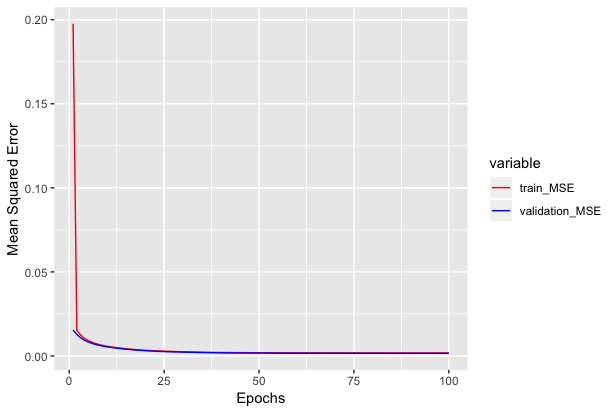
+We can see how mean squared error varies with epochs below.
+
+<!--notebook-skip-line-->
+
+Inference on the network
+---------
+Now we have trained the network. Let's use it for inference.
+
+```r
+## We extract the state symbols for RNN
+internals <- model$symbol$get.internals()
+sym_state <- internals$get.output(which(internals$outputs %in% "RNN_state"))
+sym_state_cell <- internals$get.output(which(internals$outputs %in% "RNN_state_cell"))
+sym_output <- internals$get.output(which(internals$outputs %in% "loss_output"))
+symbol <- mx.symbol.Group(sym_output, sym_state, sym_state_cell)
+
+## We will predict 100 timestamps for 401st sample (first sample from the test samples)
+pred_length <- 100
+predicted <- numeric()
+
+## We pass the 400th sample through the network to get the weights and use it for predicting next
+## 100 time stamps.
+data <- mx.nd.array(trainX[, , 400, drop = F])
+label <- mx.nd.array(trainY[, 400, drop = F])
+
+
+## We create dataiterators for the input, please note that the label is required to create
+## iterator and will not be used in the inference. You can use dummy values too in the label.
+infer.data <- mx.io.arrayiter(data = data,
+ label = label,
+ batch.size = 1,
+ shuffle = FALSE)
+
+infer <- mx.infer.rnn.one(infer.data = infer.data,
+ symbol = symbol,
+ arg.params = model$arg.params,
+ aux.params = model$aux.params,
+ input.params = NULL,
+ ctx = ctx)
+## Once we get the weights for the above time series, we try to predict the next 100 steps for
+## this time series, which is technically our 401st time series.
+
+actual <- trainY[, 401]
+
+## Now we iterate one by one to generate each of the next timestamp pollution values
+
+for (i in 1:pred_length) {
+
+ data <- mx.nd.array(trainX[, i, 401, drop = F])
+ label <- mx.nd.array(trainY[i, 401, drop = F])
+ infer.data <- mx.io.arrayiter(data = data,
+ label = label,
+ batch.size = 1,
+ shuffle = FALSE)
+ ## note that we use rnn state values from previous iterations here
+ infer <- mx.infer.rnn.one(infer.data = infer.data,
+ symbol = symbol,
+ ctx = ctx,
+ arg.params = model$arg.params,
+ aux.params = model$aux.params,
+ input.params = list(rnn.state = infer[[2]],
+ rnn.state.cell = infer[[3]]))
+
+ pred <- infer[[1]]
+ predicted <- c(predicted, as.numeric(as.array(pred)))
+
+}
+
+```
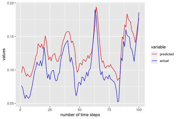
+Now predicted contains the predicted 100 values. We use ggplot to plot the actual and predicted values as shown below.
+
+<!--notebook-skip-line-->
+
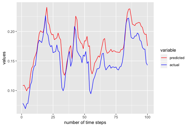
+We also repeated the above experiments to generate the next 100 samples to 301st time series and we got the following results.
+
+<!--notebook-skip-line-->
+
+The above tutorial is just for demonstration purposes and has not been tuned extensively for accuracy.
+
+For more tutorials on MXNet-R, head on to [MXNet-R tutorials](https://mxnet.incubator.apache.org/tutorials/r/index.html)
\ No newline at end of file
diff --git a/docs/tutorials/r/MultidimLstm.md b/docs/tutorials/r/MultidimLstm.md
new file mode 100644
index 00000000000..8692086d180
--- /dev/null
+++ b/docs/tutorials/r/MultidimLstm.md
@@ -0,0 +1,302 @@
+LSTM time series example
+=============================================
+
+This tutorial shows how to use an LSTM model with multivariate data, and generate predictions from it. For demonstration purposes, we used an open source [pollution data](https://archive.ics.uci.edu/ml/datasets/Beijing+PM2.5+Data).
+The tutorial is an illustration of how to use LSTM models with MXNet-R. We are forecasting the air pollution with data recorded at the US embassy in Beijing, China for five years.
+
+Dataset Attribution:
+"PM2.5 data of US Embassy in Beijing"
+We want to predict pollution levels(PM2.5 concentration) in the city given the above dataset.
+
+```r
+Dataset description:
+No: row number
+year: year of data in this row
+month: month of data in this row
+day: day of data in this row
+hour: hour of data in this row
+pm2.5: PM2.5 concentration
+DEWP: Dew Point
+TEMP: Temperature
+PRES: Pressure
+cbwd: Combined wind direction
+Iws: Cumulated wind speed
+Is: Cumulated hours of snow
+Ir: Cumulated hours of rain
+```
+
+We use past PM2.5 concentration, dew point, temperature, pressure, wind speed, snow and rain to predict
+PM2.5 concentration levels.
+
+Load and pre-process the data
+---------
+The first step is to load in the data and preprocess it. It is assumed that the data has been downloaded in a .csv file: data.csv from the [pollution dataset](https://archive.ics.uci.edu/ml/datasets/Beijing+PM2.5+Data)
+
+ ```r
+## Loading required packages
+library("readr")
+library("dplyr")
+library("mxnet")
+library("abind")
+ ```
+
+
+
+ ```r
+## Preprocessing steps
+Data <- read.csv(file = "/Users/khedia/Downloads/data.csv",
+ header = TRUE,
+ sep = ",")
+
+## Extracting specific features from the dataset as variables for time series We extract
+## pollution, temperature, pressue, windspeed, snowfall and rainfall information from dataset
+df <- data.frame(Data$pm2.5,
+ Data$DEWP,
+ Data$TEMP,
+ Data$PRES,
+ Data$Iws,
+ Data$Is,
+ Data$Ir)
+df[is.na(df)] <- 0
+
+## Now we normalise each of the feature set to a range(0,1)
+df <- matrix(as.matrix(df),
+ ncol = ncol(df),
+ dimnames = NULL)
+
+rangenorm <- function(x) {
+ (x - min(x))/(max(x) - min(x))
+}
+df <- apply(df, 2, rangenorm)
+df <- t(df)
+ ```
+For using multidimesional data with MXNet-R, we need to convert training data to the form
+(n_dim x seq_len x num_samples). For one-to-one RNN flavours labels should be of the form (seq_len x num_samples) while for many-to-one flavour, the labels should be of the form (1 x num_samples). Please note that MXNet-R currently supports only these two flavours of RNN.
+We have used n_dim = 7, seq_len = 100, and num_samples = 430 because the dataset has 430 samples, each the length of 100 timestamps, we have seven time series as input features so each input has dimesnion of seven at each time step.
+
+
+```r
+n_dim <- 7
+seq_len <- 100
+num_samples <- 430
+
+## extract only required data from dataset
+trX <- df[1:n_dim, 25:(24 + (seq_len * num_samples))]
+
+## the label data(next PM2.5 concentration) should be one time step
+## ahead of the current PM2.5 concentration
+trY <- df[1, 26:(25 + (seq_len * num_samples))]
+
+## reshape the matrices in the format acceptable by MXNetR RNNs
+trainX <- trX
+dim(trainX) <- c(n_dim, seq_len, num_samples)
+trainY <- trY
+dim(trainY) <- c(seq_len, num_samples)
+```
+
+
+
+Defining and training the network
+---------
+
+```r
+batch.size <- 32
+
+# take first 300 samples for training - remaining 100 for evaluation
+train_ids <- 1:300
+eval_ids <- 301:400
+
+## The number of samples used for training and evaluation is arbitrary. I have kept aside few
+## samples for testing purposes create dataiterators
+train.data <- mx.io.arrayiter(data = trainX[, , train_ids, drop = F],
+ label = trainY[, train_ids],
+ batch.size = batch.size, shuffle = TRUE)
+
+eval.data <- mx.io.arrayiter(data = trainX[, , eval_ids, drop = F],
+ label = trainY[, eval_ids],
+ batch.size = batch.size, shuffle = FALSE)
+
+## Create the symbol for RNN
+symbol <- rnn.graph(num_rnn_layer = 1,
+ num_hidden = 5,
+ input_size = NULL,
+ num_embed = NULL,
+ num_decode = 1,
+ masking = F,
+ loss_output = "linear",
+ dropout = 0.2,
+ ignore_label = -1,
+ cell_type = "lstm",
+ output_last_state = T,
+ config = "one-to-one")
+
+
+
+mx.metric.mse.seq <- mx.metric.custom("MSE", function(label, pred) {
+ label = mx.nd.reshape(label, shape = -1)
+ pred = mx.nd.reshape(pred, shape = -1)
+ res <- mx.nd.mean(mx.nd.square(label - pred))
+ return(as.array(res))
+})
+
+
+
+ctx <- mx.cpu()
+
+initializer <- mx.init.Xavier(rnd_type = "gaussian",
+ factor_type = "avg",
+ magnitude = 3)
+
+optimizer <- mx.opt.create("adadelta",
+ rho = 0.9,
+ eps = 1e-05,
+ wd = 1e-06,
+ clip_gradient = 1,
+ rescale.grad = 1/batch.size)
+
+logger <- mx.metric.logger()
+epoch.end.callback <- mx.callback.log.train.metric(period = 10,
+ logger = logger)
+
+## train the network
+system.time(model <- mx.model.buckets(symbol = symbol,
+ train.data = train.data,
+ eval.data = eval.data,
+ num.round = 100,
+ ctx = ctx,
+ verbose = TRUE,
+ metric = mx.metric.mse.seq,
+ initializer = initializer,
+ optimizer = optimizer,
+ batch.end.callback = NULL,
+ epoch.end.callback = epoch.end.callback))
+```
+Output:
+```
+Start training with 1 devices
+[1] Train-MSE=0.197570244409144
+[1] Validation-MSE=0.0153861071448773
+[2] Train-MSE=0.0152517843060195
+[2] Validation-MSE=0.0128299412317574
+[3] Train-MSE=0.0124418652616441
+[3] Validation-MSE=0.010827143676579
+[4] Train-MSE=0.0105128229130059
+[4] Validation-MSE=0.00940261723008007
+[5] Train-MSE=0.00914482437074184
+[5] Validation-MSE=0.00830172537826002
+[6] Train-MSE=0.00813581114634871
+[6] Validation-MSE=0.00747016374953091
+[7] Train-MSE=0.00735094994306564
+[7] Validation-MSE=0.00679832429159433
+[8] Train-MSE=0.00672049634158611
+[8] Validation-MSE=0.00623159145470709
+[9] Train-MSE=0.00620287149213254
+[9] Validation-MSE=0.00577476259786636
+[10] Train-MSE=0.00577280316501856
+[10] Validation-MSE=0.00539038667920977
+..........
+..........
+[91] Train-MSE=0.00177705133100972
+[91] Validation-MSE=0.00154715491225943
+[92] Train-MSE=0.00177639147732407
+[92] Validation-MSE=0.00154592350008897
+[93] Train-MSE=0.00177577760769054
+[93] Validation-MSE=0.00154474508599378
+[94] Train-MSE=0.0017752077546902
+[94] Validation-MSE=0.0015436161775142
+[95] Train-MSE=0.00177468206966296
+[95] Validation-MSE=0.00154253660002723
+[96] Train-MSE=0.00177419915562496
+[96] Validation-MSE=0.00154150440357625
+[97] Train-MSE=0.0017737578949891
+[97] Validation-MSE=0.00154051734716631
+[98] Train-MSE=0.00177335749613121
+[98] Validation-MSE=0.00153957353904843
+[99] Train-MSE=0.00177299699280411
+[99] Validation-MSE=0.00153867155313492
+[100] Train-MSE=0.00177267640829086
+[100] Validation-MSE=0.00153781197150238
+
+ user system elapsed
+ 21.937 1.914 13.402
+```
+We can see how mean squared error varies with epochs below.
+
+<!--notebook-skip-line-->
+
+Inference on the network
+---------
+Now we have trained the network. Let's use it for inference.
+
+```r
+## We extract the state symbols for RNN
+internals <- model$symbol$get.internals()
+sym_state <- internals$get.output(which(internals$outputs %in% "RNN_state"))
+sym_state_cell <- internals$get.output(which(internals$outputs %in% "RNN_state_cell"))
+sym_output <- internals$get.output(which(internals$outputs %in% "loss_output"))
+symbol <- mx.symbol.Group(sym_output, sym_state, sym_state_cell)
+
+## We will predict 100 timestamps for 401st sample (first sample from the test samples)
+pred_length <- 100
+predicted <- numeric()
+
+## We pass the 400th sample through the network to get the weights and use it for predicting next
+## 100 time stamps.
+data <- mx.nd.array(trainX[, , 400, drop = F])
+label <- mx.nd.array(trainY[, 400, drop = F])
+
+
+## We create dataiterators for the input, please note that the label is required to create
+## iterator and will not be used in the inference. You can use dummy values too in the label.
+infer.data <- mx.io.arrayiter(data = data,
+ label = label,
+ batch.size = 1,
+ shuffle = FALSE)
+
+infer <- mx.infer.rnn.one(infer.data = infer.data,
+ symbol = symbol,
+ arg.params = model$arg.params,
+ aux.params = model$aux.params,
+ input.params = NULL,
+ ctx = ctx)
+## Once we get the weights for the above time series, we try to predict the next 100 steps for
+## this time series, which is technically our 401st time series.
+
+actual <- trainY[, 401]
+
+## Now we iterate one by one to generate each of the next timestamp pollution values
+
+for (i in 1:pred_length) {
+
+ data <- mx.nd.array(trainX[, i, 401, drop = F])
+ label <- mx.nd.array(trainY[i, 401, drop = F])
+ infer.data <- mx.io.arrayiter(data = data,
+ label = label,
+ batch.size = 1,
+ shuffle = FALSE)
+ ## note that we use rnn state values from previous iterations here
+ infer <- mx.infer.rnn.one(infer.data = infer.data,
+ symbol = symbol,
+ ctx = ctx,
+ arg.params = model$arg.params,
+ aux.params = model$aux.params,
+ input.params = list(rnn.state = infer[[2]],
+ rnn.state.cell = infer[[3]]))
+
+ pred <- infer[[1]]
+ predicted <- c(predicted, as.numeric(as.array(pred)))
+
+}
+
+```
+Now predicted contains the predicted 100 values. We use ggplot to plot the actual and predicted values as shown below.
+
+<!--notebook-skip-line-->
+
+We also repeated the above experiments to generate the next 100 samples to 301st time series and we got the following results.
+
+<!--notebook-skip-line-->
+
+The above tutorial is just for demonstration purposes and has not been tuned extensively for accuracy.
+
+For more tutorials on MXNet-R, head on to [MXNet-R tutorials](https://mxnet.incubator.apache.org/tutorials/r/index.html)
\ No newline at end of file
diff --git a/tests/tutorials/test_sanity_tutorials.py b/tests/tutorials/test_sanity_tutorials.py
index f9fb0ac2c49..cd3f6bfcbac 100644
--- a/tests/tutorials/test_sanity_tutorials.py
+++ b/tests/tutorials/test_sanity_tutorials.py
@@ -42,6 +42,7 @@
'r/fiveMinutesNeuralNetwork.md',
'r/index.md',
'r/mnistCompetition.md',
+ 'r/MultidimLstm.md',
'r/ndarray.md',
'r/symbol.md',
'scala/char_lstm.md',
----------------------------------------------------------------
This is an automated message from the Apache Git Service.
To respond to the message, please log on GitHub and use the
URL above to go to the specific comment.
For queries about this service, please contact Infrastructure at:
users@infra.apache.org
With regards,
Apache Git Services